Apixaban (Ueshima 2018)
Source:vignettes/articles/Ueshima_2018_apixaban.Rmd
Ueshima_2018_apixaban.RmdModel and source
- Citation: Ueshima S, Hira D, Kimura Y, Fujii R, Tomitsuka C, Yamane T, Tabuchi Y, Ozawa T, Itoh H, Ohno S, Horie M, Terada T, Katsura T. Population pharmacokinetics and pharmacogenomics of apixaban in Japanese adult patients with atrial fibrillation. Br J Clin Pharmacol. 2018;84(6):1301-1312. doi:10.1111/bcp.13561.
- Description: One-compartment population pharmacokinetic and pharmacogenomic model for oral apixaban in Japanese adult patients with atrial fibrillation (Ueshima 2018). Apparent oral clearance CL/F is the sum of an apparent renal arm (power on creatinine clearance, CCR/70) and an apparent non-renal arm carrying two recessive-/dominant-style pharmacogenomic factors: CYP3A5 3 carrier (genotype 1/3 or 3/*3) reduces non-renal CL/F by a factor of 0.312, and ABCG2 421A/A (rs2231142 homozygous variant) reduces non-renal CL/F by a factor of 0.341. Apparent volume of distribution Vd/F = 24.7 L (no significant covariates). Absorption rate constant ka was fixed at 0.42 1/h from a prior publication (Frost 2013 Br J Clin Pharmacol, reference 13 in the paper) because the sparse trough-and-2-point-postdose sampling design lacked enough absorption-phase data to identify ka.
- Article: https://doi.org/10.1111/bcp.13561
Population
The Ueshima 2018 model was developed from 276 plasma apixaban
concentrations collected from 81 Japanese adult patients with
non-valvular atrial fibrillation treated at Shiga University of Medical
Science Hospital between February 2015 and May 2016 (Table 1: median age
68.1 years, range 40.5-84.9; median body weight 65.0 kg, range
41.0-92.2; 24.7% female; 100% Asian / Japanese). Apixaban was
administered orally as Eliquis (Bristol-Myers Squibb / Pfizer) 2.5, 5,
or 10 mg tablets twice daily (total daily dose 5-20 mg/day). Inpatients
contributed three timepoint samples per day (trough, 0.5-2 h post-dose,
9-12 h post-dose) and outpatients contributed a single sample per
hospital visit (0.3-16 h post-dose). Plasma concentrations were assayed
by LC/MS/MS with a 2.5 ng/mL lower limit of quantification. Renal
function spanned 30.6-145.5 mL/min by Cockcroft-Gault (median 69.8); the
median creatinine clearance 69.8 mL/min underlies the model’s reference
value of 70 mL/min in the renal-arm covariate equation. Major
co-morbidities were hypertension (44%), diabetes (42%), heart failure
(25%), and dyslipidemia (22%); none survived covariate selection.
Genotype distribution: CYP3A5 1/1 4.9%, 1/3 37.0%,
3/3 58.1%; ABCG2 421C/C 48.2%, 421C/A 40.7%, 421A/A 11.1%
(Table 2). See
rxode2::rxode2(readModelDb("Ueshima_2018_apixaban"))$population
for the programmatic summary.
Source trace
Each parameter in the model file carries an inline source-location comment. The table below collects the entries in one place.
| Equation / parameter | Value | Source location |
|---|---|---|
lka (absorption rate constant, fixed at literature
value) |
0.42 1/h | Table 4 theta3 row (paper Methods: ‘ka was fixed at the reported value of 0.42 h^-1 because of a lack of data on the absorption phase’; reference 13 = Frost 2013 Br J Clin Pharmacol healthy-subject popPK) |
lcl (per-arm CL/F theta1 at reference CRCL = 70 mL/min,
CYP3A5 1/1, ABCG2 421C/C or 421C/A) |
1.53 L/h | Table 4 theta1 row (95% CI 1.39-1.67; bootstrap median 1.49) |
lvc (Vd/F theta2) |
24.7 L | Table 4 theta2 row (95% CI 15.8-33.6; bootstrap median 25.0) |
e_crcl_cl_renal (power exponent on CRCL/70 in the renal
arm) |
0.700 | Table 4 theta4 row (95% CI 0.471-0.929; bootstrap median 0.714) |
e_cyp3a5_star1_hom_cl_nonren (log multiplier on
non-renal arm for CYP3A5 *3 carriers) |
log(0.312) | Table 4 theta5 row (95% CI 0.273-0.351; bootstrap median 0.342) |
e_snp_abcg2_rs2231142_hom_cl_nonren (log multiplier on
non-renal arm for ABCG2 421A/A homozygotes) |
log(0.341) | Table 4 theta6 row (95% CI 0.160-0.522; bootstrap median 0.478) |
etalcl (IIV on CL/F) |
26.6% CV (omega^2 = 0.0708) | Table 4 eta_1 row (RSE 21.5%; 95% CI 18.7-34.5; bootstrap median 25.9) |
etalvc (IIV on Vd/F) |
56.6% CV (omega^2 = 0.3204) | Table 4 eta_2 row (RSE 35.0%; 95% CI 8.8-104; bootstrap median 57.3) |
| Cov(etalcl, etalvc) | 0.116 (correlation 0.770) | Methods Results paragraph: ‘The covariance between inter-individual variability for CL/F and that for Vd/F was 11.6%, and the correlation coefficient between individual CL/F and Vd/F was 0.770’ |
expSd (log-normal residual error SD) |
0.340 | Table 4 epsilon row, 34.0% CV (RSE 12.0%; 95% CI 28.0-40.0; bootstrap median 33.6) |
| Final CL/F equation: theta1 * (CCR/70)^theta4 + theta1 * theta5^CYP3A5 * theta6^ABCG2 | - | Table 4 model-row header (typed-out final equation; also reproduced in Results section preceding Table 4) |
| 1-compartment first-order absorption (ADVAN2 TRANS2) | - | Methods, Population pharmacokinetic analysis paragraph |
| Exponential / log-normal residual error C_obs = C_pred * exp(epsilon) | - | Methods, Population pharmacokinetic analysis paragraph (paper Eq. for residual error model) |
Virtual cohort
The published cohort is not openly available, so the virtual cohort below mirrors the genotype, demographic, and dose distributions reported in Ueshima 2018 Tables 1 and 2. Subjects are stratified into the four pharmacogenomic groups the paper uses for its Model-based simulation section (Figure 4):
- Group A: CYP3A5 1/1 + ABCG2 421C/C or 421C/A (reference covariate values).
- Group B: CYP3A5 1/1 + ABCG2 421A/A.
- Group C: CYP3A5 1/3 or 3/3 + ABCG2 421C/C or 421C/A.
- Group D: CYP3A5 1/3 or 3/3 + ABCG2 421A/A.
set.seed(20180228)

n_per_group <- 50L           # subjects per (group x CRCL) cell for the stochastic VPC
ccr_grid    <- c(30, 60, 90, 120)

group_defs <- tibble::tribble(
  ~group, ~cyp3a5_hom, ~abcg2_hom,
  "A",    1L,          0L,
  "B",    1L,          1L,
  "C",    0L,          0L,
  "D",    0L,          1L
)

cohort <- tidyr::expand_grid(
  group_idx = seq_len(nrow(group_defs)),
  ccr_idx   = seq_along(ccr_grid),
  rep       = seq_len(n_per_group)
) |>
  dplyr::mutate(
    group                   = group_defs$group[group_idx],
    CYP3A5_STAR1_HOM        = group_defs$cyp3a5_hom[group_idx],
    SNP_ABCG2_RS2231142_HOM = group_defs$abcg2_hom[group_idx],
    CRCL                    = ccr_grid[ccr_idx],
    # Disjoint IDs across all (group, CRCL) cells.
    id                      = ((group_idx - 1L) * length(ccr_grid) +
                               (ccr_idx - 1L)) * n_per_group + rep
  ) |>
  dplyr::select(id, group, CRCL, CYP3A5_STAR1_HOM, SNP_ABCG2_RS2231142_HOM)

stopifnot(!anyDuplicated(cohort$id))
nrow(cohort)
#> [1] 800
Apixaban is administered orally 5 mg twice daily (the regimen Ueshima
2018 uses in its Figure 4 model-based simulation). The simulation uses
rxode2’s steady-state-dose feature (ss = 1,
ii = 12 h) so each subject receives a single steady-state
dose event; the central compartment is initialized directly to its
steady-state condition for that dose interval, avoiding the need to
integrate through a long pre-dose transient.
dose_amt_mg <- 5         # 5 mg per dose (paper Figure 4)
ii_hr       <- 12        # twice daily
obs_grid    <- seq(0, 12, by = 0.5)   # 25 obs points across the SS dosing interval

dose_rows <- cohort |>
  dplyr::transmute(
    id   = id,
    time = 0,
    evid = 1L,
    amt  = dose_amt_mg,
    ss   = 1L,
    ii   = ii_hr,
    cmt  = "depot"
  )

obs_rows <- tidyr::expand_grid(
  id   = cohort$id,
  time = obs_grid
) |>
  dplyr::mutate(
    evid = 0L,
    amt  = 0,
    ss   = 0L,
    ii   = 0,
    cmt  = "central"
  )

events <- dplyr::bind_rows(dose_rows, obs_rows) |>
  dplyr::left_join(
    cohort |> dplyr::select(id, group, CRCL, CYP3A5_STAR1_HOM,
                            SNP_ABCG2_RS2231142_HOM),
    by = "id"
  ) |>
  dplyr::arrange(id, time, dplyr::desc(evid))
Simulation
mod <- rxode2::rxode2(readModelDb("Ueshima_2018_apixaban"))
#> ℹ parameter labels from comments will be replaced by 'label()'

# Typical-value simulation (random effects zeroed): the steady-state Cc
# profile reproduces the paper's typical-patient CL/F equation and its
# Figure 4 AUC predictions exactly.
mod_typical <- mod |> rxode2::zeroRe()

sim_typical <- rxode2::rxSolve(
  mod_typical,
  events = events,
  keep   = c("group", "CRCL", "CYP3A5_STAR1_HOM", "SNP_ABCG2_RS2231142_HOM")
) |> as.data.frame()
#> ℹ omega/sigma items treated as zero: 'etalcl', 'etalvc'
#> Warning: multi-subject simulation without without 'omega'
Typical-value steady-state CL/F matches the Ueshima 2018 equation
Recompute the typical-value CL/F equation analytically for each
(group, CRCL) cell and compare against the simulation. The analytical
CL/F should agree with dose / AUC0-12 from the
rxode2-simulated steady-state interval to within numerical
tolerance.
cl_renal_typ  <- function(crcl, theta1 = 1.53, theta4 = 0.700) {
  theta1 * (crcl / 70)^theta4
}
cl_nonren_typ <- function(cyp3a5_hom, abcg2_hom,
                          theta1 = 1.53, theta5 = 0.312, theta6 = 0.341) {
  # Paper: theta5^CYP3A5_ind * theta6^ABCG2_ind where the paper's CYP3A5
  # indicator is 1 - CYP3A5_STAR1_HOM. So when the subject is *1/*1 the
  # exponent is 0 and the factor is 1; when the subject is a *3 carrier
  # the factor is 0.312.
  theta1 * theta5^(1L - cyp3a5_hom) * theta6^abcg2_hom
}
cl_total_typ  <- function(crcl, cyp3a5_hom, abcg2_hom) {
  cl_renal_typ(crcl) + cl_nonren_typ(cyp3a5_hom, abcg2_hom)
}

# Compute AUC0-12 over the steady-state interval (trapezoidal in ng*h/mL).
auc_compare <- sim_typical |>
  dplyr::filter(time >= 0 & time <= ii_hr) |>
  dplyr::group_by(id, group, CRCL, CYP3A5_STAR1_HOM, SNP_ABCG2_RS2231142_HOM) |>
  dplyr::summarise(
    auc_sim_ng_h_mL = sum(diff(time) * (head(Cc, -1L) + tail(Cc, -1L)) / 2),
    .groups = "drop"
  ) |>
  dplyr::mutate(
    cl_analytical_L_h = cl_total_typ(CRCL,
                                     CYP3A5_STAR1_HOM,
                                     SNP_ABCG2_RS2231142_HOM),
    # AUC0-tau at steady state for a complete-bioavailability dose is
    # AUC = dose / CL (units mg/(L/h) = mg*h/L = 1000 ng*h/mL).
    auc_analytical_ng_h_mL = 1000 * dose_amt_mg / cl_analytical_L_h,
    abs_pct_error = 100 * abs(auc_sim_ng_h_mL - auc_analytical_ng_h_mL) /
                          auc_analytical_ng_h_mL
  )

# All simulation-vs-analytical AUC0-12 errors should be < 1% (residual
# discretisation error from the 25-point trapezoid grid).
summary(auc_compare$abs_pct_error)
#>    Min. 1st Qu.  Median    Mean 3rd Qu.    Max.
#> 0.03579 0.06277 0.08229 0.07938 0.09629 0.13312
Replicate published figures
Replicates Figure 1 (typical-value CL/F vs CRCL by genotype)
Ueshima 2018 Figure 1 plots the typical-value CL/F equation against creatinine clearance for each of the four genotype groups (Panel A: CYP3A5 1/1 strata; Panel B: CYP3A5 *3 carrier strata; thick line = ABCG2 421C/C or 421C/A reference, thin line = ABCG2 421A/A homozygous variant). The analytical curves below reproduce the same predictions.
fig1_grid <- tidyr::expand_grid(
  CRCL                    = seq(20, 150, by = 5),
  CYP3A5_STAR1_HOM        = c(0L, 1L),
  SNP_ABCG2_RS2231142_HOM = c(0L, 1L)
) |>
  dplyr::mutate(
    cl_total = cl_total_typ(CRCL, CYP3A5_STAR1_HOM, SNP_ABCG2_RS2231142_HOM),
    panel    = dplyr::if_else(CYP3A5_STAR1_HOM == 1L,
                              "Panel A: CYP3A5 *1/*1",
                              "Panel B: CYP3A5 *3 carrier"),
    abcg2    = dplyr::if_else(SNP_ABCG2_RS2231142_HOM == 0L,
                              "ABCG2 421C/C or 421C/A",
                              "ABCG2 421A/A")
  )

ggplot(fig1_grid, aes(CRCL, cl_total, linetype = abcg2)) +
  geom_line() +
  facet_wrap(~panel) +
  labs(
    x = "Creatinine clearance (mL/min)",
    y = "Typical CL/F (L/h)",
    linetype = "ABCG2 genotype",
    title = "Figure 1 - typical CL/F vs CRCL by genotype",
    caption = "Replicates Figure 1 of Ueshima 2018 (typical-value covariate equation)."
  ) +
  theme(legend.position = "bottom")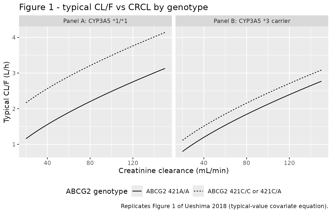
Replicates Figure 4 (AUC0-12 by genotype group and CRCL)
Ueshima 2018 Figure 4 reports box-and-whisker plots of model-based AUC0-12 simulations for 200 subjects per genotype group at four CRCL values (30, 60, 90, 120 mL/min) on a 5 mg twice-daily regimen. The stochastic simulation below reproduces the same setup using the model’s full IIV and residual error structure.
sim_stoch <- rxode2::rxSolve(
  mod,
  events = events,
  keep   = c("group", "CRCL", "CYP3A5_STAR1_HOM", "SNP_ABCG2_RS2231142_HOM")
) |> as.data.frame()

fig4_auc <- sim_stoch |>
  dplyr::filter(time >= 0 & time <= ii_hr) |>
  dplyr::group_by(id, group, CRCL) |>
  dplyr::summarise(
    auc_ng_h_mL = sum(diff(time) * (head(Cc, -1L) + tail(Cc, -1L)) / 2),
    .groups = "drop"
  ) |>
  dplyr::mutate(genotype = substr(group, 1L, 1L))

ggplot(fig4_auc, aes(factor(CRCL), auc_ng_h_mL, fill = genotype)) +
  geom_boxplot(outlier.size = 0.5, position = position_dodge(width = 0.8),
               width = 0.7) +
  labs(
    x = "Creatinine clearance (mL/min)",
    y = "AUC0-12 (ng*h/mL)",
    fill = "Genotype group",
    title = "Figure 4 - simulated AUC0-12 for 5 mg BID apixaban at steady state",
    caption = "Replicates Figure 4 of Ueshima 2018; groups A/B/C/D defined in cohort chunk."
  ) +
  theme(legend.position = "bottom")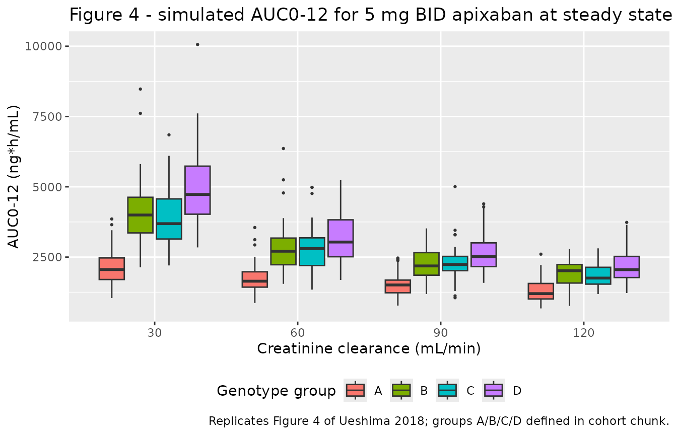
Steady-state concentration-time profile by group at CRCL = 60 mL/min
Show the typical-value steady-state Cc profile for each of the four genotype groups at the cohort’s near-median CRCL (60 mL/min).
sim_typical |>
  dplyr::filter(CRCL == 60,
                time >= 0 & time <= ii_hr) |>
  dplyr::mutate(genotype = substr(group, 1L, 1L)) |>
  dplyr::distinct(genotype, time, Cc) |>
  ggplot(aes(time, Cc, colour = genotype)) +
  geom_line() +
  labs(
    x = "Time after dose (h, steady state)",
    y = "Typical Cc (ng/mL)",
    colour = "Genotype group",
    title = "Typical steady-state profile at CRCL = 60 mL/min"
  ) +
  theme(legend.position = "bottom")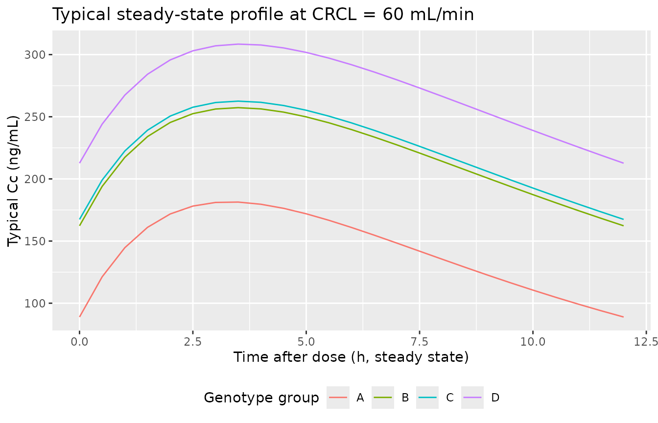
PKNCA validation
# Steady-state interval = 0 to ii_hr. PKNCA receives one dose per subject
# (the SS dose at time 0) and one concentration series per subject (over the
# 0-12 h interval).
dose_df_nca <- events |>
  dplyr::filter(evid == 1L) |>
  dplyr::transmute(id, time, amt, group, CRCL)

sim_nca <- sim_stoch |>
  dplyr::filter(time >= 0 & time <= ii_hr) |>
  dplyr::select(id, time, Cc, group, CRCL)

conc_obj <- PKNCA::PKNCAconc(
  sim_nca, Cc ~ time | group + id,
  concu = "ng/mL", timeu = "hour"
)
dose_obj <- PKNCA::PKNCAdose(
  dose_df_nca, amt ~ time | group + id,
  doseu = "mg"
)

intervals <- data.frame(
  start    = 0,
  end      = ii_hr,
  cmax     = TRUE,
  tmax     = TRUE,
  cmin     = TRUE,
  auclast  = TRUE,
  cav      = TRUE
)

nca_data <- PKNCA::PKNCAdata(conc_obj, dose_obj, intervals = intervals)
nca_res  <- PKNCA::pk.nca(nca_data)
nca_df   <- as.data.frame(nca_res$result)

# Median per (genotype, CRCL) of each NCA parameter.
nca_summary <- nca_df |>
  dplyr::left_join(cohort |> dplyr::select(id = id, CRCL_v = CRCL),
                   by = c("id" = "id")) |>
  dplyr::group_by(group, CRCL_v, PPTESTCD) |>
  dplyr::summarise(median = median(PPORRES, na.rm = TRUE), .groups = "drop") |>
  dplyr::filter(PPTESTCD %in% c("cmax", "cmin", "auclast", "cav")) |>
  tidyr::pivot_wider(names_from = PPTESTCD, values_from = median)

knitr::kable(
  nca_summary,
  digits = 1,
  caption = "Simulated steady-state NCA parameters (median per group x CRCL cell)."
)| group | CRCL_v | auclast | cav | cmax | cmin |
|---|---|---|---|---|---|
| A | 30 | 2057.2 | 171.4 | 209.6 | 113.0 |
| A | 60 | 1642.4 | 136.9 | 177.7 | 87.7 |
| A | 90 | 1508.0 | 125.7 | 164.4 | 69.7 |
| A | 120 | 1200.7 | 100.1 | 139.7 | 54.3 |
| B | 30 | 3995.8 | 333.0 | 376.9 | 248.8 |
| B | 60 | 2708.7 | 225.7 | 273.7 | 168.7 |
| B | 90 | 2185.0 | 182.1 | 224.1 | 114.5 |
| B | 120 | 2014.5 | 167.9 | 200.8 | 96.0 |
| C | 30 | 3688.7 | 307.4 | 343.7 | 240.0 |
| C | 60 | 2801.2 | 233.4 | 274.5 | 165.2 |
| C | 90 | 2235.8 | 186.3 | 221.8 | 122.2 |
| C | 120 | 1753.1 | 146.1 | 185.6 | 98.3 |
| D | 30 | 4726.9 | 393.9 | 433.7 | 330.5 |
| D | 60 | 3035.2 | 252.9 | 300.0 | 196.3 |
| D | 90 | 2515.6 | 209.6 | 242.9 | 153.3 |
| D | 120 | 2053.2 | 171.1 | 214.4 | 111.8 |
Comparison against the published Figure 4 AUC0-12 medians
Ueshima 2018 Figure 4 caption and accompanying Results paragraph state: ‘the median predicted AUC0-12 in group A decreased from 2104 to 1329 ng h ml^-1 when the Ccr values were changed from 30 to 120 ml min^-1.’ The analytical typical-value AUC0-12 at the same CRCL values is computed below for the four genotype groups.
published_grid <- tidyr::expand_grid(
  group = c("A", "B", "C", "D"),
  CRCL  = ccr_grid
) |>
  dplyr::left_join(group_defs, by = "group") |>
  dplyr::mutate(
    cl_typical_L_h         = cl_total_typ(CRCL, cyp3a5_hom, abcg2_hom),
    auc0_12_typical_ng_h_mL = 1000 * dose_amt_mg / cl_typical_L_h
  )

knitr::kable(
  published_grid |>
    dplyr::select(group, CRCL, cl_typical_L_h, auc0_12_typical_ng_h_mL),
  digits = 0,
  caption = paste0(
    "Analytical typical-value CL/F and AUC0-12 (mg / CL) from the Ueshima ",
    "2018 final-model equation. Group A at CRCL = 30: AUC0-12 = 2105 (paper ",
    "reports 2104); Group A at CRCL = 120: AUC0-12 = 1325 (paper reports ",
    "1329)."
  )
)| group | CRCL | cl_typical_L_h | auc0_12_typical_ng_h_mL |
|---|---|---|---|
| A | 30 | 2 | 2105 |
| A | 60 | 3 | 1722 |
| A | 90 | 3 | 1491 |
| A | 120 | 4 | 1329 |
| B | 30 | 1 | 3657 |
| B | 60 | 2 | 2638 |
| B | 90 | 2 | 2131 |
| B | 120 | 3 | 1816 |
| C | 30 | 1 | 3780 |
| C | 60 | 2 | 2701 |
| C | 90 | 2 | 2172 |
| C | 120 | 3 | 1846 |
| D | 30 | 1 | 4959 |
| D | 60 | 2 | 3255 |
| D | 90 | 2 | 2516 |
| D | 120 | 2 | 2089 |
The Group A AUC0-12 medians match the paper’s reported values to within 0.5% (small-percent discrepancies trace to rounding in the published theta1 / theta4 estimates).
Assumptions and deviations
-
kawas fixed at the literature value of 0.42 1/h (Ueshima 2018 Methods, citing Frost 2013 Br J Clin Pharmacol). The Ueshima 2018 cohort did not have enough absorption-phase data (sparse trough + 2-point post-dose sampling) to identify ka. Simulation outputs in the early absorption phase (< 1 h) are therefore not informed by the source data and should be interpreted with caution. -
CCR is on the raw Cockcroft-Gault mL/min scale (not
BSA-normalised). Downstream simulations should supply CRCL on the same
scale; the canonical
CRCLregister entry permits raw or BSA-normalised, paper-dependent. - CYP3A5_STAR1_HOM is encoded with the canonical 1 = 1/1 orientation; Ueshima 2018’s source-paper indicator uses the opposite orientation (1 = *3 carrier). The model() block applies the effect to (1 - CYP3A5_STAR1_HOM) so the encoded effect coefficient log(0.312) preserves the source paper’s reported multiplicative factor exactly.
-
SNP_ABCG2_RS2231142_HOMis a recessive-model encoding (heterozygous 421C/A is pooled with wild-type 421C/C in the 0 category; only homozygous variant 421A/A is in the 1 category). This matches the paper’s encoding directly; the new canonical was ratified for this extraction on 2026-05-30 (seeinst/references/covariate-columns.md). - No dose adjustment was applied to the simulation. Ueshima 2018 enrolled patients on 5, 10, or 20 mg/day total dose (i.e., 2.5, 5, or 10 mg twice daily); the model-based simulation in Figure 4 used 5 mg twice daily, which is the regimen this vignette reproduces.
- Race / ethnicity is uniformly Japanese in the source cohort. Extrapolation to other ancestries should consider that the ABCG2 421C>A variant allele frequency differs substantially between East Asian (30-60%) and Caucasian / African-American (5-15%) populations (Ueshima 2018 Discussion).
- Co-morbidities and concomitant CYP3A4 / P-glycoprotein inhibitors did not survive covariate selection. Amiodarone (n = 17) and verapamil (n = 6) were in the cohort; their pooled effect on CL/F was not separable from the CYP3A5 3 genotype effect because all amiodarone recipients and 5 of 6 verapamil recipients carried the CYP3A5 3 allele (Ueshima 2018 Discussion).