Nafamostat in ECMO patients, central-vein and circuit samples (Lee 2025)
Source:vignettes/articles/Lee_2025_nafamostat.Rmd
Lee_2025_nafamostat.RmdModel and source
Lee 2025 fitted two population PK/PD models to the same 24 adults on ECMO who received a continuous infusion of nafamostat mesylate into the ECMO drainage line upstream of the pump. Blood was drawn at the same times from two sites: the patient’s central venous catheter (the “patient model”) and the ECMO circuit at the oxygenator outflow (the “ECMO model”). Each site was fitted separately with a two-compartment PK model and an indirect-response model in which nafamostat inhibits the first-order loss of the activated partial thromboplastin time (aPTT). The two fits are packaged as two models:
Lee_2025_nafamostat_patient– central-venous samples.Lee_2025_nafamostat_circuit– ECMO-circuit samples.Citation: Lee DH, Lee JH, Jang JH, Kim YK, Kang G, Jung SY, Her M, Jang HJ. (2025). Pharmacokinetic and pharmacodynamic analyses of nafamostat in ECMO patients: comparing central vein and ECMO machine samples. Front Pharmacol 16:1541131. doi:10.3389/fphar.2025.1541131.
mod_patient <- readModelDb("Lee_2025_nafamostat_patient")
mod_circuit <- readModelDb("Lee_2025_nafamostat_circuit")
Population
The study enrolled 24 adults (17 male, 7 female) on VA-ECMO (n = 13) or VV-ECMO (n = 11) at Haeundae Paik Hospital, Busan, Republic of Korea, between July 2021 and October 2022 (Lee 2025 Table 1). Mean age was 60.3 years (SD 12.1) and mean weight 70.3 kg (SD 15.7). The commonest primary diagnoses were pneumonia (n = 10), cardiogenic shock or ventricular fibrillation (n = 4) and trauma (n = 4); 7 patients were also on CRRT. Nafamostat mesylate was started at 15 mg/h without a bolus and titrated to an aPTT of 40-80 s; the individual profiles of Figure 1 show rates of 15, 30 and 45 mg/h. The ECMO sweep-gas flow rate had a median of 3.75 L/min (IQR 2.5-5.5), which is the centring value of the gas-flow covariate in both models. The PK analysis used 162 central-venous and 162 ECMO-circuit concentrations, and the PD analysis 95 aPTT values from each site.
The same information is available programmatically via
mod_patient()$population.
Source trace
Every ini() value carries an in-file comment naming its
source. The table collects them. Inter-individual variability is
reported in Tables 2 and 3 as a percentage; footnote b of both tables
gives the RSE “for standard deviation”, so the percentage is the
standard deviation of eta times 100 and the variance is (percent /
100)^2.
| Quantity | Patient model | ECMO (circuit) model | Source |
|---|---|---|---|
lcl (CL, L/h) |
189 | 85.2 | Table 2 |
lvc (V1, L) |
7.01 | 3.83 | Table 2 |
lq (Q, L/h) |
350 (fixed) | 46.7 | Table 2, footnote a |
lvp (V2, L) |
55.0 | 36.8 | Table 2 |
e_qecmogas_vp (gas flow on V2) |
-0.852 | – | Table 2; Results equation for V2 |
e_qecmogas_cl (gas flow on CL) |
– | 0.0999 | Table 2; Results equation for CL |
limax (Imax) |
0.355 | 0.436 | Table 3 |
lic50 (IC50, ug/L) |
350 (fixed) | 581 (fixed) | Table 3, footnote a |
lkin (Kin, s/h) |
47.5 | 50.6 | Table 3 |
lrbase (Base, s) |
34.5 | 33.0 | Table 3 |
etalcl |
61.3% -> 0.3758 | 29.5% -> 0.0870 | Table 2 |
etalvc |
69.5% (fixed) -> 0.4830 | 62.8% (fixed) -> 0.3944 | Table 2 |
etalq |
243% (fixed) -> 5.905 | 134% (fixed) -> 1.796 | Table 2 |
etalvp |
49.2% (fixed) -> 0.2421 | 0 (fixed) | Table 2 |
etalimax |
50.7% (fixed) -> 0.2570 | 27.3% (fixed) -> 0.0745 | Table 3 |
etalic50 |
70.6% (fixed) -> 0.4984 | 0 (fixed) | Table 3, row “omegaEC50” |
etalkin |
105% -> 1.1025 | 75.8% -> 0.5746 | Table 3 |
etalrbase |
20.7% -> 0.0428 | 21.2% -> 0.0449 | Table 3 |
propSd (concentration) |
0.287 | 0.309 | Table 2 |
addSd_aPTT (s) |
2.83 | 3.43 | Table 3 |
Two-compartment PK, infusion into central
|
– | – | Methods 2.4 (ADVAN3 TRANS4); Results 3.3 |
V2 = thetaV2 * exp(theta * (gas flow - 3.75)) |
yes | – | Results 3.3, first equation |
CL = thetaCL * exp(theta * (gas flow - 3.75)) |
– | yes | Results 3.3, second equation |
d/dt(aPTT) = Kin - Kout * (1 - Imax*Cp/(IC50 + Cp)) * aPTT,
Kout = Kin / Base, aPTT(0) = Base
|
yes | yes | Results 3.3, turnover equations |
Closed-form checks of the packaged parameters
Two deterministic checks tie the packaged typical values to statements in the paper. Neither depends on a random draw.
Distribution and elimination half-lives. The Discussion reports t1/2alpha = 0.54 min and t1/2beta = 19.7 min for the patient model, and 1.2 min and 51.4 min for the ECMO model. They follow from the Table 2 typical values through the usual two-compartment eigenvalues.
two_cmt_half_lives <- function(cl, vc, q, vp) {
  k10 <- cl / vc
  k12 <- q / vc
  k21 <- q / vp
  s <- k10 + k12 + k21
  disc <- sqrt(s^2 - 4 * k10 * k21)
  # minutes
  60 * log(2) / c(alpha = (s + disc) / 2, beta = (s - disc) / 2)
}
typ <- function(mod) {
  th <- rxode2::rxode(mod)$theta
  exp(th[c("lcl", "lvc", "lq", "lvp")])
}
tp <- typ(mod_patient)
#> ℹ parameter labels from comments will be replaced by 'label()'
tc <- typ(mod_circuit)
#> ℹ parameter labels from comments will be replaced by 'label()'
hl <- rbind(
  patient = two_cmt_half_lives(tp[["lcl"]], tp[["lvc"]], tp[["lq"]], tp[["lvp"]]),
  circuit = two_cmt_half_lives(tc[["lcl"]], tc[["lvc"]], tc[["lq"]], tc[["lvp"]])
)
hl_pub <- rbind(patient = c(alpha = 0.54, beta = 19.7), circuit = c(alpha = 1.2, beta = 51.4))
data.frame(
  model = rownames(hl),
  alpha_model = round(hl[, "alpha"], 2),
  alpha_paper = hl_pub[, "alpha"],
  beta_model = round(hl[, "beta"], 1),
  beta_paper = hl_pub[, "beta"]
) |>
  dplyr::rename(
    "Model" = model,
    "t1/2 alpha, packaged (min)" = alpha_model,
    "t1/2 alpha, Discussion (min)" = alpha_paper,
    "t1/2 beta, packaged (min)" = beta_model,
    "t1/2 beta, Discussion (min)" = beta_paper
  ) |>
knitr::kable(row.names = FALSE, caption = "Half-lives from the packaged Table 2 values vs. the Discussion of Lee 2025.")| Model | t1/2 alpha, packaged (min) | t1/2 alpha, Discussion (min) | t1/2 beta, packaged (min) | t1/2 beta, Discussion (min) |
|---|---|---|---|---|
| patient | 0.51 | 0.54 | 19.7 | 19.7 |
| circuit | 1.19 | 1.20 | 51.4 | 51.4 |
stopifnot(
  # beta reproduces to the printed precision in both models
  all(abs(hl[, "beta"] / hl_pub[, "beta"] - 1) < 0.01),
  # alpha is printed to two significant figures; the patient value computes
  # to 0.51 min against the printed 0.54
  all(abs(hl[, "alpha"] / hl_pub[, "alpha"] - 1) < 0.1)
)
Steady-state concentration and aPTT. For a
continuous infusion into the central compartment the steady-state
concentration is R / CL, and the turnover model settles at
aPTT = Base / (1 - Imax * C / (IC50 + C)). The
typical-value solve below confirms both at the end of a 24-h infusion at
30 mg/h with the sweep-gas flow at its 3.75 L/min reference. (After the
6-h infusions of Figure 3 the ECMO model is still about 0.5% below its
plateau, because its terminal half-life is 51 min.)
ev_typ <- rxode2::et(amt = 30 * 6, rate = 30, cmt = "central") |>
  rxode2::et(seq(0, 8, by = 0.05), cmt = "aPTT") |>
  as.data.frame() |>
  dplyr::mutate(Q_ECMO_GAS = 3.75)
ev_long <- rxode2::et(amt = 30 * 24, rate = 30, cmt = "central") |>
  rxode2::et(c(0, 23.99), cmt = "aPTT") |>
  as.data.frame() |>
  dplyr::mutate(Q_ECMO_GAS = 3.75)
typ_ss <- function(mod) {
  s <- rxode2::rxSolve(rxode2::zeroRe(mod), ev_long, rtol = 1e-10, atol = 1e-12, returnType = "data.frame")
  s[abs(s$time - 23.99) < 1e-9, c("Cc", "aPTT")]
}
th_p <- exp(rxode2::rxode(mod_patient)$theta)
#> ℹ parameter labels from comments will be replaced by 'label()'
th_c <- exp(rxode2::rxode(mod_circuit)$theta)
#> ℹ parameter labels from comments will be replaced by 'label()'
closed <- function(th) {
  css <- 1000 * 30 / th[["lcl"]]
  c(Cc = css, aPTT = th[["lrbase"]] / (1 - th[["limax"]] * css / (th[["lic50"]] + css)))
}
ss_chk <- rbind(
  patient = c(unlist(typ_ss(mod_patient)), closed(th_p)),
  circuit = c(unlist(typ_ss(mod_circuit)), closed(th_c))
)
#> ℹ parameter labels from comments will be replaced by 'label()'
#> ℹ omega/sigma items treated as zero: 'etalcl', 'etalvc', 'etalq', 'etalvp', 'etalimax', 'etalic50', 'etalkin', 'etalrbase'
#> ℹ parameter labels from comments will be replaced by 'label()'
#> ℹ omega/sigma items treated as zero: 'etalcl', 'etalvc', 'etalq', 'etalvp', 'etalimax', 'etalic50', 'etalkin', 'etalrbase'
colnames(ss_chk) <- c("Cc_solve", "aPTT_solve", "Cc_closed", "aPTT_closed")
knitr::kable(signif(ss_chk, 4), caption = "Typical-value solve at the end of a 24-h infusion vs. closed form, 30 mg/h.")| Cc_solve | aPTT_solve | Cc_closed | aPTT_closed | |
|---|---|---|---|---|
| patient | 158.7 | 38.8 | 158.7 | 38.8 |
| circuit | 352.1 | 39.5 | 352.1 | 39.5 |
stopifnot(
  # 24 h is > 28 terminal half-lives in both models, so the residual
  # approach term is < 1e-8 and the bound is set by the solver tolerance
  all(abs(ss_chk[, "Cc_solve"] / ss_chk[, "Cc_closed"] - 1) < 1e-3),
  # turnover t1/2 = log(2) * Base / Kin is about 0.5 h in both models
  all(abs(ss_chk[, "aPTT_solve"] / ss_chk[, "aPTT_closed"] - 1) < 1e-3)
)
Virtual cohort and simulation
Figure 3 of Lee 2025 shows median concentration and aPTT from 2,000 virtual patients per model over a 6-h infusion at 10, 20, 30, 40 and 50 mg/h. Here each model is simulated with 200 virtual patients per infusion rate, with between-subject and residual variability. The paper does not say how the sweep-gas flow covariate was set for the simulation; it is held at the 3.75 L/min cohort median.
rates <- c(10, 20, 30, 40, 50)
n_per_arm <- 200L
obs_times <- seq(0, 8, by = 0.05)

make_arm <- function(rate_mgh, n, id_offset) {
  ids <- id_offset + seq_len(n)
  label <- paste(rate_mgh, "mg/h")
  dose <- data.frame(
    id = ids, time = 0, evid = 1L, amt = rate_mgh * 6, rate = rate_mgh,
    cmt = "central"
  )
  obs <- tidyr::expand_grid(id = ids, time = obs_times) |>
    dplyr::mutate(evid = 0L, amt = NA_real_, rate = NA_real_, cmt = "aPTT")
  dplyr::bind_rows(dose, obs) |>
    dplyr::mutate(Q_ECMO_GAS = 3.75, dose_rate = label) |>
    dplyr::arrange(id, time, dplyr::desc(evid))
}
events <- dplyr::bind_rows(lapply(seq_along(rates), function(i) {
  make_arm(rates[i], n_per_arm, id_offset = (i - 1L) * n_per_arm)
}))
stopifnot(!anyDuplicated(unique(events[, c("id", "time", "evid")])))
rxode2::rxSetSeed(20250521)
sim_one <- function(mod, label) {
  rxode2::rxSolve(mod, events = events, keep = "dose_rate", returnType = "data.frame") |>
    dplyr::mutate(model = label)
}
sim <- dplyr::bind_rows(
  sim_one(mod_patient, "Patient model"),
  sim_one(mod_circuit, "ECMO model")
) |>
  dplyr::mutate(dose_rate = factor(dose_rate, levels = paste(rates, "mg/h")))
#> ℹ parameter labels from comments will be replaced by 'label()'
#> ℹ parameter labels from comments will be replaced by 'label()'
#> ℹ omega/sigma items treated as zero: 'etalvp', 'etalic50'
stopifnot(!anyNA(sim$dose_rate), nlevels(droplevels(sim$dose_rate)) == length(rates))
Replicate Figure 3
fig3 <- sim |>
  dplyr::group_by(model, dose_rate, time) |>
  dplyr::summarise(
    `Concentration (ug/L)` = median(Cc),
    `aPTT (s)` = median(aPTT),
    .groups = "drop"
  ) |>
  tidyr::pivot_longer(c(`Concentration (ug/L)`, `aPTT (s)`), names_to = "output", values_to = "median")
ggplot(fig3, aes(time, median, colour = dose_rate)) +
  geom_line() +
  facet_grid(output ~ model, scales = "free_y") +
  labs(
    x = "Time (h)", y = "Median of 200 virtual patients", colour = "Infusion rate",
    caption = "Replicates Figure 3 of Lee 2025 with the parameters of Tables 2 and 3."
  ) +
  theme_bw() +
  theme(legend.position = "bottom")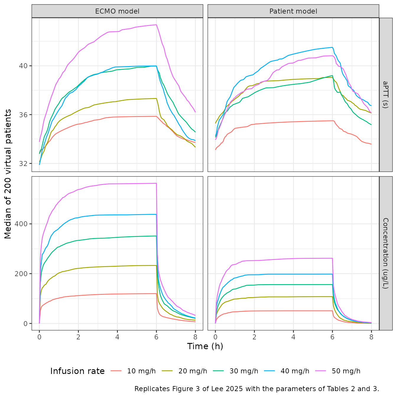
Figure 3 concentrations do not follow from Table 2
The aPTT panels above resemble Figure 3, but the concentration
plateaus do not. The paper’s text reports a median steady-state
concentration at 30 mg/h of about 88 ug/L in the patient model and about
600 ug/L in the ECMO model; with the Table 2 clearances the plateau is
R / CL = 159 ug/L and 352 ug/L. The mismatch runs in
opposite directions in the two models, so it is not a unit or salt-form
factor (salt-to-base conversion would lower both).
The plateaus in Figure 3 are instead reproduced, for every infusion
rate and both models, by R / Q: the Figure 3 simulation
appears to have used the intercompartmental clearance (350 and 46.7 L/h)
in place of the clearance (189 and 85.2 L/h). Table 2 as printed is
supported by everything else in the paper: the Results text quotes CL =
189 and 85.2 L/h; the Discussion half-lives above reproduce only with
the Table 2 assignment (with CL and Q exchanged the ECMO t1/2beta
becomes 53.0 min instead of the printed 51.4); and the observed circuit
concentrations of Figure 1 at the 15 mg/h starting rate, mostly 80-250
ug/L, bracket R / CL = 176 ug/L and lie below
R / Q = 321 ug/L. (The central-venous observations at 15
mg/h, mostly 20-100 ug/L, are compatible with either 79 or 43 ug/L.) The
packaged models therefore keep Table 2 as printed.
The plateau values below were read from Figure 3 by the maintainers (the 30 mg/h values are the ones stated in the Results text).
fig3_read <- tibble::tribble(
  ~model, ~rate, ~css_fig3,
  "Patient model", 10, 30,
  "Patient model", 20, 57,
  "Patient model", 30, 88,
  "Patient model", 40, 119,
  "Patient model", 50, 145,
  "ECMO model", 10, 205,
  "ECMO model", 20, 435,
  "ECMO model", 30, 600,
  "ECMO model", 40, 790,
  "ECMO model", 50, 1030
)
pk_typ <- tibble::tibble(
  model = c("Patient model", "ECMO model"),
  cl = c(th_p[["lcl"]], th_c[["lcl"]]),
  q = c(th_p[["lq"]], th_c[["lq"]])
)
plateau <- fig3_read |>
  dplyr::left_join(pk_typ, by = "model") |>
  dplyr::mutate(
    css_table2 = 1000 * rate / cl,
    css_swapped = 1000 * rate / q,
    ratio_table2 = css_table2 / css_fig3,
    ratio_swapped = css_swapped / css_fig3
  )
plateau |>
  dplyr::transmute(
    model, rate,
    css_fig3, css_table2 = round(css_table2), css_swapped = round(css_swapped)
  ) |>
  dplyr::rename(
    "Model" = model,
    "Rate (mg/h)" = rate,
    "Figure 3 plateau (ug/L)" = css_fig3,
    "R / CL, Table 2 (ug/L)" = css_table2,
    "R / Q (ug/L)" = css_swapped
  ) |>
knitr::kable(caption = "Steady-state concentration: Figure 3 vs. the packaged clearance and vs. the intercompartmental clearance.")| Model | Rate (mg/h) | Figure 3 plateau (ug/L) | R / CL, Table 2 (ug/L) | R / Q (ug/L) |
|---|---|---|---|---|
| Patient model | 10 | 30 | 53 | 29 |
| Patient model | 20 | 57 | 106 | 57 |
| Patient model | 30 | 88 | 159 | 86 |
| Patient model | 40 | 119 | 212 | 114 |
| Patient model | 50 | 145 | 265 | 143 |
| ECMO model | 10 | 205 | 117 | 214 |
| ECMO model | 20 | 435 | 235 | 428 |
| ECMO model | 30 | 600 | 352 | 642 |
| ECMO model | 40 | 790 | 469 | 857 |
| ECMO model | 50 | 1030 | 587 | 1071 |
stopifnot(
  # R / Q reproduces every Figure 3 plateau to within the reading precision
  all(abs(plateau$ratio_swapped - 1) < 0.12),
  # ...and R / CL misses every one of them by more than 40%, in opposite
  # directions in the two models
  all(abs(plateau$ratio_table2 - 1) > 0.4)
)
The simulated median aPTT at 6 h is compared with the Results text below. Because Figure 3’s concentrations were simulated with a different clearance, its aPTT curves are not an exact target either; the packaged patient model lands on the stated 39 s, while the packaged ECMO model gives about 40 s against the stated 43 s, consistent with its lower simulated concentration.
sim |>
  dplyr::filter(dose_rate == "30 mg/h", abs(time - 6) < 1e-9) |>
  dplyr::group_by(model) |>
  dplyr::summarise(cc = median(Cc), aptt = median(aPTT), .groups = "drop") |>
  dplyr::left_join(
    tibble::tibble(model = c("Patient model", "ECMO model"), cc_pub = c(88, 600), aptt_pub = c(39, 43)),
    by = "model"
  ) |>
  dplyr::mutate(cc = round(cc), aptt = round(aptt, 1)) |>
  dplyr::rename(
    "Model" = model,
    "Simulated median Cc at 6 h (ug/L)" = cc,
    "Simulated median aPTT at 6 h (s)" = aptt,
    "Paper Cc (ug/L)" = cc_pub,
    "Paper aPTT (s)" = aptt_pub
  ) |>
knitr::kable(caption = "30 mg/h: simulated medians vs. Results section 3.3 of Lee 2025.")| Model | Simulated median Cc at 6 h (ug/L) | Simulated median aPTT at 6 h (s) | Paper Cc (ug/L) | Paper aPTT (s) |
|---|---|---|---|---|
| ECMO model | 351 | 40.0 | 600 | 43 |
| Patient model | 156 | 39.2 | 88 | 39 |
Effect of the sweep-gas flow covariate
In the patient model the sweep-gas flow lowers the peripheral volume,
which changes only the approach to steady state; in the ECMO model it
raises clearance, so the plateau falls by
exp(-0.0999 * (gas - 3.75)).
# Typical-value solves over several covariate levels are multi-subject solves
# of a zeroRe() model, so rxode2 notes that there is no omega; that note is
# expected here and muffled.
muffle_no_omega <- function(w) {
  if (grepl("without 'omega'", conditionMessage(w), fixed = TRUE)) invokeRestart("muffleWarning")
}
solve_typical <- function(mod, events, ...) {
  withCallingHandlers(
    rxode2::rxSolve(rxode2::zeroRe(mod), events, keep = "Q_ECMO_GAS", returnType = "data.frame", ...),
    warning = muffle_no_omega
  )
}
gas_levels <- c(2.5, 3.75, 5.5)
ev_gas <- dplyr::bind_rows(lapply(seq_along(gas_levels), function(i) {
  ev_typ |> dplyr::mutate(id = i, Q_ECMO_GAS = gas_levels[i])
}))
gas_sim <- dplyr::bind_rows(
  solve_typical(mod_patient, ev_gas) |>
    dplyr::mutate(model = "Patient model"),
  solve_typical(mod_circuit, ev_gas) |>
    dplyr::mutate(model = "ECMO model")
)
#> ℹ parameter labels from comments will be replaced by 'label()'
#> ℹ omega/sigma items treated as zero: 'etalcl', 'etalvc', 'etalq', 'etalvp', 'etalimax', 'etalic50', 'etalkin', 'etalrbase'
#> ℹ parameter labels from comments will be replaced by 'label()'
#> ℹ omega/sigma items treated as zero: 'etalcl', 'etalvc', 'etalq', 'etalvp', 'etalimax', 'etalic50', 'etalkin', 'etalrbase'
ggplot(gas_sim, aes(time, Cc, colour = factor(Q_ECMO_GAS))) +
  geom_line() +
  facet_wrap(~model, scales = "free_y") +
  labs(
    x = "Time (h)", y = "Typical Cc (ug/L)", colour = "Sweep gas (L/min)",
    caption = "30 mg/h for 6 h at the Table 1 quartiles and median of sweep-gas flow."
  ) +
  theme_bw()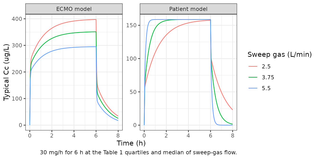
# plateau check on a 24-h infusion (the 6-h run above is ~0.5% short of it)
gas_ss <- dplyr::bind_rows(lapply(seq_along(gas_levels), function(i) {
  ev_long |> dplyr::mutate(id = i, Q_ECMO_GAS = gas_levels[i])
})) |>
  solve_typical(mod = mod_circuit, rtol = 1e-10, atol = 1e-12) |>
  dplyr::filter(abs(time - 23.99) < 1e-9) |>
  dplyr::arrange(Q_ECMO_GAS)
#> ℹ parameter labels from comments will be replaced by 'label()'
#> ℹ omega/sigma items treated as zero: 'etalcl', 'etalvc', 'etalq', 'etalvp', 'etalimax', 'etalic50', 'etalkin', 'etalrbase'
stopifnot(all(abs(gas_ss$Cc / (1000 * 30 / (th_c[["lcl"]] * exp(0.0999 * (gas_levels - 3.75)))) - 1) < 1e-3))
PKNCA validation
The paper reports no NCA. PKNCA is run on the simulated cohorts to summarise the plateau (average concentration from 2 to 6 h, after steady state) and the post-infusion half-life, and the plateau is compared with Figure 3. Every row is expected to differ by more than 20% for the reason explained above; the comparison is shown so the size of that discrepancy is visible next to the simulated values.
sim_nca <- sim |>
  dplyr::filter(!is.na(Cc)) |>
  dplyr::mutate(treatment = paste(model, dose_rate, sep = ", ")) |>
  dplyr::select(id, time, Cc, treatment)
conc_obj <- PKNCA::PKNCAconc(sim_nca, Cc ~ time | treatment + id)
#> Warning in assert_conc(conc, any_missing_conc = any_missing_conc): Negative
#> concentrations found
dose_df <- events |>
  dplyr::filter(evid == 1) |>
  dplyr::select(id, time, amt, dose_rate)
dose_df <- dplyr::bind_rows(
  dose_df |> dplyr::mutate(treatment = paste("Patient model", dose_rate, sep = ", ")),
  dose_df |> dplyr::mutate(treatment = paste("ECMO model", dose_rate, sep = ", "))
) |>
  dplyr::select(id, time, amt, treatment)
dose_obj <- PKNCA::PKNCAdose(dose_df, amt ~ time | treatment + id, duration = 6)
intervals <- data.frame(
  start = c(2, 6),
  end = c(6, 8),
  cav = c(TRUE, FALSE),
  cmax = c(TRUE, FALSE),
  half.life = c(FALSE, TRUE)
)
nca_res <- PKNCA::pk.nca(PKNCA::PKNCAdata(conc_obj, dose_obj, intervals = intervals))
#> Warning in assert_conc(conc, any_missing_conc = any_missing_conc): Negative
#> concentrations found
#> Warning in assert_conc(conc, any_missing_conc = any_missing_conc): Negative
#> concentrations found
#> Warning in assert_conc(conc, any_missing_conc = any_missing_conc): Negative
#> concentrations found
#> Warning in assert_conc(conc, any_missing_conc = any_missing_conc): Negative
#> concentrations found
#> Warning in log(data$conc): NaNs produced
#> Warning in assert_conc(conc, any_missing_conc = any_missing_conc): Negative
#> concentrations found
#> Warning in assert_conc(conc, any_missing_conc = any_missing_conc): Negative
#> concentrations found
#> Warning in assert_conc(conc, any_missing_conc = any_missing_conc): Negative
#> concentrations found
#> Warning in assert_conc(conc, any_missing_conc = any_missing_conc): Negative
#> concentrations found
#> Warning in log(data$conc): NaNs produced
#> Warning in assert_conc(conc, any_missing_conc = any_missing_conc): Negative
#> concentrations found
#> Warning in assert_conc(conc, any_missing_conc = any_missing_conc): Negative
#> concentrations found
#> Warning in assert_conc(conc, any_missing_conc = any_missing_conc): Negative
#> concentrations found
#> Warning in assert_conc(conc, any_missing_conc = any_missing_conc): Negative
#> concentrations found
#> Warning in log(data$conc): NaNs produced
#> Warning in assert_conc(conc, any_missing_conc = any_missing_conc): Negative
#> concentrations found
#> Warning in assert_conc(conc, any_missing_conc = any_missing_conc): Negative
#> concentrations found
#> Warning in assert_conc(conc, any_missing_conc = any_missing_conc): Negative
#> concentrations found
#> Warning in assert_conc(conc, any_missing_conc = any_missing_conc): Negative
#> concentrations found
#> Warning in log(data$conc): NaNs produced
#> Warning in assert_conc(conc, any_missing_conc = any_missing_conc): Negative
#> concentrations found
#> Warning in assert_conc(conc, any_missing_conc = any_missing_conc): Negative
#> concentrations found
#> Warning in assert_conc(conc, any_missing_conc = any_missing_conc): Negative
#> concentrations found
#> Warning in assert_conc(conc, any_missing_conc = any_missing_conc): Negative
#> concentrations found
#> Warning in log(data$conc): NaNs produced
#> Warning in assert_conc(conc, any_missing_conc = any_missing_conc): Negative
#> concentrations found
#> Warning in assert_conc(conc, any_missing_conc = any_missing_conc): Negative
#> concentrations found
#> Warning in assert_conc(conc, any_missing_conc = any_missing_conc): Negative
#> concentrations found
#> Warning in assert_conc(conc, any_missing_conc = any_missing_conc): Negative
#> concentrations found
#> Warning in log(data$conc): NaNs produced
#> Warning in assert_conc(conc, any_missing_conc = any_missing_conc): Negative
#> concentrations found
#> Warning in assert_conc(conc, any_missing_conc = any_missing_conc): Negative
#> concentrations found
#> Warning in assert_conc(conc, any_missing_conc = any_missing_conc): Negative
#> concentrations found
#> Warning in assert_conc(conc, any_missing_conc = any_missing_conc): Negative
#> concentrations found
#> Warning in log(data$conc): NaNs produced
#> Warning in assert_conc(conc, any_missing_conc = any_missing_conc): Negative
#> concentrations found
#> Warning in assert_conc(conc, any_missing_conc = any_missing_conc): Negative
#> concentrations found
#> Warning in assert_conc(conc, any_missing_conc = any_missing_conc): Negative
#> concentrations found
#> Warning in assert_conc(conc, any_missing_conc = any_missing_conc): Negative
#> concentrations found
#> Warning in log(data$conc): NaNs produced
#> Warning in assert_conc(conc, any_missing_conc = any_missing_conc): Negative
#> concentrations found
#> Warning in assert_conc(conc, any_missing_conc = any_missing_conc): Negative
#> concentrations found
#> Warning in assert_conc(conc, any_missing_conc = any_missing_conc): Negative
#> concentrations found
#> Warning in assert_conc(conc, any_missing_conc = any_missing_conc): Negative
#> concentrations found
#> Warning in log(data$conc): NaNs produced
nca_tab <- as.data.frame(nca_res) |>
  dplyr::filter(PPTESTCD %in% c("cav", "half.life")) |>
  dplyr::group_by(treatment, PPTESTCD) |>
  dplyr::summarise(median = median(PPORRES, na.rm = TRUE), .groups = "drop") |>
  tidyr::pivot_wider(names_from = PPTESTCD, values_from = median)
nca_tab |>
  dplyr::mutate(cav = round(cav), half.life = round(60 * half.life, 1)) |>
  dplyr::rename(
    "Model, rate" = treatment,
    "Median Cav 2-6 h (ug/L)" = cav,
    "Median post-infusion t1/2 (min)" = half.life
  ) |>
knitr::kable(caption = "PKNCA summary of the simulated cohorts.")| Model, rate | Median Cav 2-6 h (ug/L) | Median post-infusion t1/2 (min) |
|---|---|---|
| ECMO model, 10 mg/h | 118 | 54.6 |
| ECMO model, 20 mg/h | 229 | 54.2 |
| ECMO model, 30 mg/h | 344 | 57.9 |
| ECMO model, 40 mg/h | 435 | 56.4 |
| ECMO model, 50 mg/h | 561 | 49.3 |
| Patient model, 10 mg/h | 51 | 26.3 |
| Patient model, 20 mg/h | 107 | 27.1 |
| Patient model, 30 mg/h | 156 | 25.4 |
| Patient model, 40 mg/h | 199 | 26.0 |
| Patient model, 50 mg/h | 259 | 26.2 |
published <- fig3_read |>
  dplyr::transmute(treatment = paste(model, paste(rate, "mg/h"), sep = ", "), cav = css_fig3)
cmp <- nlmixr2lib::ncaComparisonTable(
  simulated = nca_res,
  reference = published,
  by = "treatment",
  params = "cav",
  units = c(cav = "ug/L"),
  tolerance_pct = 20
)
knitr::kable(cmp, caption = "Simulated plateau vs. Figure 3 of Lee 2025. * differs from reference by >20% (expected; see text).")| NCA parameter | treatment | Reference | Simulated | % diff |
|---|---|---|---|---|
| Cavg (ug/L) | Patient model, 10 mg/h | 30 | 50.8 | +69.4%* |
| Cavg (ug/L) | Patient model, 20 mg/h | 57 | 107 | +87.3%* |
| Cavg (ug/L) | Patient model, 30 mg/h | 88 | 156 | +77.5%* |
| Cavg (ug/L) | Patient model, 40 mg/h | 119 | 199 | +67.2%* |
| Cavg (ug/L) | Patient model, 50 mg/h | 145 | 259 | +78.9%* |
| Cavg (ug/L) | ECMO model, 10 mg/h | 205 | 118 | -42.6%* |
| Cavg (ug/L) | ECMO model, 20 mg/h | 435 | 229 | -47.3%* |
| Cavg (ug/L) | ECMO model, 30 mg/h | 600 | 344 | -42.7%* |
| Cavg (ug/L) | ECMO model, 40 mg/h | 790 | 435 | -44.9%* |
| Cavg (ug/L) | ECMO model, 50 mg/h | 1030 | 561 | -45.6%* |
The Cav medians track R / CL of the packaged models (the
median of R / CL_i equals R / CL for a
log-normal clearance), so the starred rows are the Figure 3 discrepancy,
not a simulation artefact.
cav_chk <- nca_tab |>
  dplyr::mutate(
    model = sub(",.*$", "", treatment),
    rate = as.numeric(sub("^.*, ([0-9]+) mg/h$", "\\1", treatment))
  ) |>
  dplyr::left_join(pk_typ, by = "model") |>
  dplyr::mutate(ratio = cav / (1000 * rate / cl))
stopifnot(
  # median over 200 subjects of R / CL_i: omega_CL = 0.613 gives a sampling
  # SD of the median of about 5.4%, so 20% is > 3.5 SE
  all(abs(cav_chk$ratio - 1) < 0.2)
)
Assumptions and deviations
- Figure 3 is not reproduced as published. Its concentration plateaus equal infusion rate / Q rather than infusion rate / CL in both models (see above). The packaged models keep Table 2 as printed, because the Results text, the Discussion half-lives and the observed concentrations in Figure 1 all agree with it.
- IIV scale. Tables 2 and 3 give IIV as a percentage with the RSE footnoted “for standard deviation”; the percentage is taken as the standard deviation of eta times 100, so variance = (percent / 100)^2. The bootstrap intervals are percentile intervals and cannot distinguish this from a log-normal CV reading; under the CV reading the large values (Q: 243% and 134%; Kin: 105%) would give much smaller variances.
- ECMO-model IIV of Kin. Table 3 prints 75.8% with no RSE and no bootstrap interval, and does not mark it as fixed; it is packaged as an estimated variance.
-
Zero variances. The ECMO model’s IIV on V2 and on
IC50 are printed as 0.000 (fixed); they are packaged as
fixed(0)etas so the parameter set mirrors the table. -
Table 3 row label. The row “omegaEC50” is the IIV
of IC50 (the model has no EC50); it is packaged as
etalic50. - Imax above 1. Imax carries exponential IIV as printed. A virtual subject whose individual Imax * C / (IC50 + C) exceeds 1 has a negative aPTT loss rate and an aPTT that rises without limit during the infusion. At the infusion rates of Figure 3 this needs an eta several standard deviations out, so it is rare, but users simulating much higher concentrations should check for it.
- Sweep-gas flow. The paper does not say whether the covariate was time-varying within a patient, nor what value its Figure 3 simulation used; it is held at the 3.75 L/min cohort median here.
- Dosing site. Nafamostat was infused into the ECMO drainage line upstream of the pump. Both models, as in the paper, treat the infusion as an input to the central compartment; the difference between the sampling sites is carried entirely by the separately estimated parameters.
- Sequential PK/PD. The paper fixed each patient’s empirical Bayes PK parameters while estimating the PD parameters. The packaged models join the PK and PD layers in one model with independent etas, which is the simulation-equivalent form.
- No erratum or correction notice for this article was found in Europe PMC or PubMed as of 2026-11-04.