Vancomycin (Smit 2021)

Model and source

• Citation: Smit C, Goulooze SC, Bruggemann RJM, Sherwin CM, Knibbe CAJ. Dosing Recommendations for Vancomycin in Children and Adolescents with Varying Levels of Obesity and Renal Dysfunction: a Population Pharmacokinetic Study in 1892 Children Aged 1-18 Years. AAPS J. 2021;23(3):53. doi:10.1208/s12248-021-00577-x
• Description: Two-compartment IV population PK model for vancomycin in normal-weight, overweight and obese children and adolescents aged 1-18 years with a wide range of renal function (Smit 2021). Clearance scales as a power function of total body weight (estimated exponent 0.745, reference 22.1 kg) and linearly with bedside-Schwartz creatinine clearance capped at 120 mL/min/1.73 m^2 (reference 100 mL/min/1.73 m^2); central and peripheral volumes scale linearly with total body weight and intercompartmental clearance as a power function of total body weight (exponent 0.599). Residual variability is additive on log-transformed concentrations.
• Article: https://doi.org/10.1208/s12248-021-00577-x
• Supplement (methods, results, NONMEM control stream of the final model): Online Resource 1 at the article landing page.

Smit 2021 is a retrospective multicenter population PK analysis of intravenous vancomycin in 1892 children and adolescents aged 1-18 years, 548 of whom were overweight or obese, with renal function spanning a bedside Schwartz creatinine clearance of 8.6 to over 900 mL/min/1.73 m^2. The final two-compartment model (Table II) drives clearance by total body weight (power function, estimated exponent 0.745) and by bedside Schwartz CLcr (linear, capped at 120 mL/min/1.73 m^2). The paper then uses the typical-value model to derive a weight- and renal-function-based dosing guideline (Table III) and demonstrates it on six typical individuals (Figure 4). This vignette reproduces Figure 4 numerically from the packaged model.

Population

The analysis used routine therapeutic-drug-monitoring data from 21 Intermountain Healthcare hospitals in Utah, USA, collected between 2006 and 2012 (Smit 2021 Methods; Table I). Of 1924 eligible patients, 26 on renal replacement therapy or ECMO and 6 without a recorded body weight were excluded, leaving 1892 patients and 5524 serum concentrations: 1344 normal weight, 247 overweight and 301 obese (BMI-for-age above the 85th and 95th percentile of the WHO (1-2 years) or CDC (2-18 years) charts). Median age was about 7 years in each weight group (range 1-18); median total body weight was 20.6, 25.0 and 30.0 kg in the three groups (overall range 5.8-188 kg). About 56% were male and 88% Caucasian; 35% were admitted to intensive care and about 17% were neutropenic. Median bedside Schwartz CLcr was 111.7-121.2 mL/min/1.73 m^2 across weight groups; only 12 patients were below 30 mL/min/1.73 m^2. Vancomycin was generally dosed at 15-20 mg/kg two to four times daily as 60-min infusions.

The same information is available programmatically via the model’s population metadata (readModelDb("Smit_2021_vancomycin")()$population).

Source trace

Per-parameter origin is recorded as an in-file comment next to each ini() entry in inst/modeldb/specificDrugs/Smit_2021_vancomycin.R. The table below collects them in one place.

Equation / parameter	Value	Source location
lcl (CL at 22.1 kg, CLcr 100)	2.12 L/h (RSE 1%)	Table II, TVCL
lvc (V1 at 22.1 kg)	8.90 L (RSE 3%)	Table II, TVV1
lq (Q at 22.1 kg)	1.55 L/h (RSE 5%)	Table II, TVQ (the table prints the unit as “L”; Q is a clearance, L/h)
lvp (V2 at 22.1 kg)	12.3 L (RSE 6%)	Table II, TVV2
e_wt_cl	0.745 (RSE 2%)	Table II, theta1
e_wt_q	0.599 (RSE 9%)	Table II, theta2
e_wt_vc_vp	1, fixed	Table II equations TVV1 x (TBW/22.1), TVV2 x (TBW/22.1); supplement control stream THETA(7) = (1) FIX
e_crcl_cl	1, fixed	Table II equation TVCL x (TBW/22.1)^theta1 x (SCHW/100); supplement control stream THETA(5) = (1) FIX
CLcr cap	120 mL/min/1.73 m^2	Table II footnote a; control stream IF(SCHW.GT.120) SCHW_MAX=120
etalcl	log(1 + 0.287^2) = 0.0792	Table II, IIV CL 28.7%; footnote c defines CV = sqrt(exp(omega^2) - 1)
etalvp	log(1 + 1.10^2) = 0.793	Table II, IIV V2 110%
cov(etalcl, etalvp)	-0.085	Table II, covariance IIV CL-V2
expSd	sqrt(0.0789) = 0.281	Table II, proportional error 0.0789 (read as the log-domain variance; see Assumptions)
Two-compartment ODE	n/a	Supplement control stream $SUBROUTINE ADVAN3 TRANS4
Residual model	n/a	Supplement control stream $ERROR: Y = LOG(F) + ERR(1) on log-transformed DV

Replicate Figure 4: the proposed dosing guideline in six typical individuals

Figure 4 of Smit 2021 simulates the Table III dosing guideline in six typical individuals from the dataset (1 year / 11 kg, 9 years / 46 kg, 12 years / 25 kg, 13 years / 78 kg, 16 years / 63 kg and 17 years / 118 kg), each at four bedside Schwartz CLcr values (10, 40, 70 and 120 mL/min/1.73 m^2), without between-subject or residual variability. Each panel prints AUCday3 (AUC from 48 to 72 h), Cmin at day 3 and AUCday1 (AUC from 0 to 24 h). Age does not enter the model; only weight and CLcr do.

Table III maps weight and CLcr to a regimen:

CLcr (mL/min/1.73 m^2)	TBW < 30 kg	TBW 30-70 kg	TBW > 70 kg
> 90	15 mg/kg q6h	15 mg/kg q8h	18 mg/kg q12h
50-90	11 mg/kg q6h (a)	11 mg/kg q8h (a)	12 mg/kg q12h (a)
30-50	5 mg/kg q6h (a)	5 mg/kg q8h (a)	6 mg/kg q12h (a)
10-30	5 mg/kg q12h (a)	3 mg/kg q12h (a)	3 mg/kg q12h (a)

1. First dose is 15 mg/kg.

fig4_individuals <- tibble::tribble(
  ~individual,                          ~WT,
  "1 year - 11 kg - normal weight",      11,
  "9 year - 46 kg - morbidly obese",     46,
  "12 year - 25 kg - normal weight",     25,
  "13 year - 78 kg - morbidly obese",    78,
  "16 year - 63 kg - normal weight",     63,
  "17 year - 118 kg - morbidly obese",  118
)

# Table III: maintenance dose (mg/kg) and interval (h) by CLcr row and weight column.
table3 <- tibble::tribble(
  ~CRCL, ~wt_band, ~dose_mgkg, ~tau, ~footnote_a,
  120,   "<30",    15,         6,    FALSE,
  120,   "30-70",  15,         8,    FALSE,
  120,   ">70",    18,         12,   FALSE,
  70,    "<30",    11,         6,    TRUE,
  70,    "30-70",  11,         8,    TRUE,
  70,    ">70",    12,         12,   TRUE,
  40,    "<30",    5,          6,    TRUE,
  40,    "30-70",  5,          8,    TRUE,
  40,    ">70",    6,          12,   TRUE,
  10,    "<30",    5,          12,   TRUE,
  10,    "30-70",  3,          12,   TRUE,
  10,    ">70",    3,          12,   TRUE
)

fig4_scenarios <- tidyr::crossing(fig4_individuals, CRCL = c(10, 40, 70, 120)) |>
  dplyr::mutate(wt_band = dplyr::case_when(WT < 30 ~ "<30", WT <= 70 ~ "30-70", TRUE ~ ">70")) |>
  dplyr::left_join(table3, by = c("CRCL", "wt_band")) |>
  dplyr::mutate(
    id = dplyr::row_number(),
    scenario = paste0(individual, " | CLcr ", CRCL),
    # Footnote (a) rows start with 15 mg/kg; the > 90 row has no footnote, so
    # its first dose is the maintenance dose.
    first_mgkg = ifelse(footnote_a, 15, dose_mgkg)
  )
knitr::kable(
  fig4_scenarios |>
    dplyr::select(individual, WT, CRCL, first_mgkg, dose_mgkg, tau) |>
    dplyr::rename(
      "Individual" = individual, "TBW (kg)" = WT, "CLcr" = CRCL,
      "First dose (mg/kg)" = first_mgkg, "Maintenance (mg/kg)" = dose_mgkg,
      "Interval (h)" = tau
    ),
  caption = "The 24 Figure 4 scenarios and their Table III regimens."
)

The 24 Figure 4 scenarios and their Table III regimens.

Individual	TBW (kg)	CLcr	First dose (mg/kg)	Maintenance (mg/kg)	Interval (h)
1 year - 11 kg - normal weight	11	10	15	5	12
1 year - 11 kg - normal weight	11	40	15	5	6
1 year - 11 kg - normal weight	11	70	15	11	6
1 year - 11 kg - normal weight	11	120	15	15	6
12 year - 25 kg - normal weight	25	10	15	5	12
12 year - 25 kg - normal weight	25	40	15	5	6
12 year - 25 kg - normal weight	25	70	15	11	6
12 year - 25 kg - normal weight	25	120	15	15	6
13 year - 78 kg - morbidly obese	78	10	15	3	12
13 year - 78 kg - morbidly obese	78	40	15	6	12
13 year - 78 kg - morbidly obese	78	70	15	12	12
13 year - 78 kg - morbidly obese	78	120	18	18	12
16 year - 63 kg - normal weight	63	10	15	3	12
16 year - 63 kg - normal weight	63	40	15	5	8
16 year - 63 kg - normal weight	63	70	15	11	8
16 year - 63 kg - normal weight	63	120	15	15	8
17 year - 118 kg - morbidly obese	118	10	15	3	12
17 year - 118 kg - morbidly obese	118	40	15	6	12
17 year - 118 kg - morbidly obese	118	70	15	12	12
17 year - 118 kg - morbidly obese	118	120	18	18	12
9 year - 46 kg - morbidly obese	46	10	15	3	12
9 year - 46 kg - morbidly obese	46	40	15	5	8
9 year - 46 kg - morbidly obese	46	70	15	11	8
9 year - 46 kg - morbidly obese	46	120	15	15	8

Doses are infused at 10 mg/min (600 mg/h) with a minimum duration of 1 h: a dose up to 600 mg runs over 60 min, a larger dose over amt / 600 hours (see Assumptions for why).

obs_times <- round(seq(0, 96, by = 0.05), 2)
build_fig4_events <- function(sc) {
  dose_times <- seq(0, 95.99, by = sc$tau)
  amts <- c(sc$first_mgkg, rep(sc$dose_mgkg, length(dose_times) - 1)) * sc$WT
  doses <- tibble::tibble(
    id = sc$id, time = dose_times, amt = amts, rate = pmin(amts, 600),
    evid = 1L, cmt = "central"
  )
  obs <- tibble::tibble(
    id = sc$id, time = obs_times, amt = 0, rate = 0, evid = 0L, cmt = "central"
  )
  dplyr::bind_rows(doses, obs) |>
    dplyr::mutate(WT = sc$WT, CRCL = sc$CRCL, scenario = sc$scenario)
}
fig4_events <- lapply(split(fig4_scenarios, fig4_scenarios$id), build_fig4_events) |>
  dplyr::bind_rows() |>
  dplyr::arrange(id, time, dplyr::desc(evid))
stopifnot(!anyDuplicated(fig4_events[, c("id", "time", "evid")]))

mod <- readModelDb("Smit_2021_vancomycin")
mod_typical <- mod |> rxode2::zeroRe()
#> ℹ parameter labels from comments will be replaced by 'label()'
sim_fig4 <- rxode2::rxSolve(
  mod_typical,
  events = fig4_events,
  keep = c("scenario", "WT", "CRCL")
) |>
  as.data.frame() |>
  dplyr::left_join(
    fig4_scenarios |> dplyr::select(id, individual, tau),
    by = "id"
  )
#> ℹ omega/sigma items treated as zero: 'etalcl', 'etalvp'
#> Warning: multi-subject simulation without without 'omega'

(The left_join above attaches one row of per-scenario metadata per id; the id values are unique per scenario, so it cannot fan out rows.)

ggplot(sim_fig4, aes(time, Cc, colour = factor(CRCL))) +
  geom_line() +
  geom_hline(yintercept = c(10, 15), linetype = "dashed") +
  facet_wrap(~individual, ncol = 3) +
  scale_x_continuous(breaks = seq(0, 96, 24)) +
  scale_colour_manual(
    values = c(`10` = "#D7191C", `40` = "#FDAE61", `70` = "#A6D96A", `120` = "#2C7BB6")
  ) +
  labs(
    x = "Time (h)", y = "Vancomycin concentration (mg/L)",
    colour = "CLcr (Schwartz)\n(mL/min/1.73 m^2)",
    title = "Figure 4 - Table III dosing guideline in six typical individuals",
    caption = "Replicates Figure 4 of Smit 2021 (typical values, no variability)."
  ) +
  theme_bw()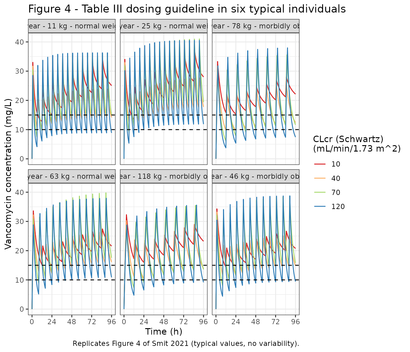

PKNCA validation against the Figure 4 labels

PKNCA computes AUCday1 (0-24 h) and AUCday3 (48-72 h) on each typical-value profile. The Figure 4 Cmin at day 3 matches the first trough after the 48 h dose (the minimum over the day-3 window once the trough at 48 h itself is excluded), so it is computed as the PKNCA cmin over 49-72 h: every dose infuses for at least 1 h and troughs rise through day 3, so that minimum is the trough at 48 h + tau.

nca_conc <- sim_fig4 |>
  dplyr::filter(!is.na(Cc)) |>
  dplyr::select(id, scenario, time, Cc)
nca_dose <- fig4_events |>
  dplyr::filter(evid == 1) |>
  dplyr::select(id, scenario, time, amt)

conc_obj <- PKNCA::PKNCAconc(nca_conc, Cc ~ time | scenario + id)
dose_obj <- PKNCA::PKNCAdose(nca_dose, amt ~ time | scenario + id)
intervals <- data.frame(
  start = c(0, 48, 49),
  end = c(24, 72, 72),
  auclast = c(TRUE, TRUE, FALSE),
  cmin = c(FALSE, FALSE, TRUE)
)
nca_res <- PKNCA::pk.nca(PKNCA::PKNCAdata(conc_obj, dose_obj, intervals = intervals))

nca_wide <- as.data.frame(nca_res) |>
  dplyr::mutate(param = dplyr::case_when(
    PPTESTCD == "auclast" & start == 0 ~ "auc_day1",
    PPTESTCD == "auclast" & start == 48 ~ "auc_day3",
    PPTESTCD == "cmin" ~ "cmin_day3"
  )) |>
  dplyr::select(scenario, param, PPORRES) |>
  tidyr::pivot_wider(names_from = param, values_from = PPORRES)

The published values below were transcribed by the maintainers from the text labels printed inside each Figure 4 panel (red = CLcr 10, orange = 40, green = 70, blue = 120 mL/min/1.73 m^2).

published_fig4 <- tibble::tribble(
  ~individual,                          ~CRCL, ~auc_day3, ~cmin_day3, ~auc_day1,
  "1 year - 11 kg - normal weight",     10,    593.45,    21.2,       420.88,
  "1 year - 11 kg - normal weight",     40,    422.52,    13.7,       373.65,
  "1 year - 11 kg - normal weight",     70,    541.09,    14.7,       415.70,
  "1 year - 11 kg - normal weight",     120,   435.02,    8.9,        355.16,
  "9 year - 46 kg - morbidly obese",    10,    496.28,    18.1,       448.20,
  "9 year - 46 kg - morbidly obese",    40,    435.67,    13.8,       398.87,
  "9 year - 46 kg - morbidly obese",    70,    565.90,    14.9,       425.38,
  "9 year - 46 kg - morbidly obese",    120,   463.76,    9.2,        363.41,
  "12 year - 25 kg - normal weight",    10,    646.89,    23.0,       453.24,
  "12 year - 25 kg - normal weight",    40,    503.07,    16.6,       420.30,
  "12 year - 25 kg - normal weight",    70,    655.77,    18.6,       478.97,
  "12 year - 25 kg - normal weight",    120,   533.20,    11.8,       418.58,
  "13 year - 78 kg - morbidly obese",   10,    521.67,    19.1,       469.74,
  "13 year - 78 kg - morbidly obese",   40,    393.37,    11.6,       377.29,
  "13 year - 78 kg - morbidly obese",   70,    463.61,    10.9,       356.34,
  "13 year - 78 kg - morbidly obese",   120,   420.97,    7.2,        334.17,
  "16 year - 63 kg - normal weight",    10,    511.40,    18.7,       460.97,
  "16 year - 63 kg - normal weight",    40,    463.01,    14.8,       417.03,
  "16 year - 63 kg - normal weight",    70,    605.87,    16.4,       448.31,
  "16 year - 63 kg - normal weight",    120,   499.53,    10.5,       385.51,
  "17 year - 118 kg - morbidly obese",  10,    541.76,    19.8,       486.35,
  "17 year - 118 kg - morbidly obese",  40,    424.72,    12.7,       399.07,
  "17 year - 118 kg - morbidly obese",  70,    505.23,    12.5,       380.20,
  "17 year - 118 kg - morbidly obese",  120,   462.88,    8.8,        360.13
) |>
  dplyr::mutate(scenario = paste0(individual, " | CLcr ", CRCL)) |>
  dplyr::select(scenario, auc_day3, cmin_day3, auc_day1)
stopifnot(nrow(published_fig4) == 24, setequal(published_fig4$scenario, nca_wide$scenario))

cmp <- nlmixr2lib::ncaComparisonTable(
  simulated = nca_wide,
  reference = published_fig4,
  by = "scenario",
  params = c("auc_day3", "cmin_day3", "auc_day1"),
  units = c(auc_day3 = "mg*h/L", cmin_day3 = "mg/L", auc_day1 = "mg*h/L"),
  tolerance_pct = 20
)
#> Warning: ncaParamLabel(): unknown PKNCA code(s) returned as-is: 'auc_day3',
#> 'cmin_day3', 'auc_day1'
knitr::kable(
  cmp,
  caption = "Simulated (PKNCA) vs. published Figure 4 values. * differs from the reference by >20%."
)

Simulated (PKNCA) vs. published Figure 4 values. * differs from the reference by >20%.

NCA parameter	scenario	Reference	Simulated	% diff
auc_day1 (mg*h/L)	1 year - 11 kg - normal weight | CLcr 10	421	421	+0.0%
auc_day1 (mg*h/L)	1 year - 11 kg - normal weight | CLcr 40	374	374	+0.0%
auc_day1 (mg*h/L)	1 year - 11 kg - normal weight | CLcr 70	416	416	+0.0%
auc_day1 (mg*h/L)	1 year - 11 kg - normal weight | CLcr 120	355	355	+0.0%
auc_day1 (mg*h/L)	9 year - 46 kg - morbidly obese | CLcr 10	448	448	+0.0%
auc_day1 (mg*h/L)	9 year - 46 kg - morbidly obese | CLcr 40	399	399	+0.0%
auc_day1 (mg*h/L)	9 year - 46 kg - morbidly obese | CLcr 70	425	425	+0.0%
auc_day1 (mg*h/L)	9 year - 46 kg - morbidly obese | CLcr 120	363	363	+0.0%
auc_day1 (mg*h/L)	12 year - 25 kg - normal weight | CLcr 10	453	453	+0.0%
auc_day1 (mg*h/L)	12 year - 25 kg - normal weight | CLcr 40	420	420	+0.0%
auc_day1 (mg*h/L)	12 year - 25 kg - normal weight | CLcr 70	479	479	+0.0%
auc_day1 (mg*h/L)	12 year - 25 kg - normal weight | CLcr 120	419	419	+0.0%
auc_day1 (mg*h/L)	13 year - 78 kg - morbidly obese | CLcr 10	470	470	+0.0%
auc_day1 (mg*h/L)	13 year - 78 kg - morbidly obese | CLcr 40	377	377	+0.0%
auc_day1 (mg*h/L)	13 year - 78 kg - morbidly obese | CLcr 70	356	356	+0.0%
auc_day1 (mg*h/L)	13 year - 78 kg - morbidly obese | CLcr 120	334	334	+0.0%
auc_day1 (mg*h/L)	16 year - 63 kg - normal weight | CLcr 10	461	461	+0.0%
auc_day1 (mg*h/L)	16 year - 63 kg - normal weight | CLcr 40	417	417	+0.0%
auc_day1 (mg*h/L)	16 year - 63 kg - normal weight | CLcr 70	448	448	+0.0%
auc_day1 (mg*h/L)	16 year - 63 kg - normal weight | CLcr 120	386	386	+0.0%
auc_day1 (mg*h/L)	17 year - 118 kg - morbidly obese | CLcr 10	486	486	+0.0%
auc_day1 (mg*h/L)	17 year - 118 kg - morbidly obese | CLcr 40	399	399	+0.0%
auc_day1 (mg*h/L)	17 year - 118 kg - morbidly obese | CLcr 70	380	380	+0.0%
auc_day1 (mg*h/L)	17 year - 118 kg - morbidly obese | CLcr 120	360	360	+0.0%
auc_day3 (mg*h/L)	1 year - 11 kg - normal weight | CLcr 10	593	594	+0.0%
auc_day3 (mg*h/L)	1 year - 11 kg - normal weight | CLcr 40	423	423	+0.0%
auc_day3 (mg*h/L)	1 year - 11 kg - normal weight | CLcr 70	541	541	+0.0%
auc_day3 (mg*h/L)	1 year - 11 kg - normal weight | CLcr 120	435	435	+0.0%
auc_day3 (mg*h/L)	9 year - 46 kg - morbidly obese | CLcr 10	496	496	+0.0%
auc_day3 (mg*h/L)	9 year - 46 kg - morbidly obese | CLcr 40	436	436	+0.0%
auc_day3 (mg*h/L)	9 year - 46 kg - morbidly obese | CLcr 70	566	566	+0.0%
auc_day3 (mg*h/L)	9 year - 46 kg - morbidly obese | CLcr 120	464	464	+0.0%
auc_day3 (mg*h/L)	12 year - 25 kg - normal weight | CLcr 10	647	647	+0.0%
auc_day3 (mg*h/L)	12 year - 25 kg - normal weight | CLcr 40	503	503	+0.0%
auc_day3 (mg*h/L)	12 year - 25 kg - normal weight | CLcr 70	656	656	+0.0%
auc_day3 (mg*h/L)	12 year - 25 kg - normal weight | CLcr 120	533	533	+0.0%
auc_day3 (mg*h/L)	13 year - 78 kg - morbidly obese | CLcr 10	522	522	+0.0%
auc_day3 (mg*h/L)	13 year - 78 kg - morbidly obese | CLcr 40	393	393	+0.0%
auc_day3 (mg*h/L)	13 year - 78 kg - morbidly obese | CLcr 70	464	464	+0.0%
auc_day3 (mg*h/L)	13 year - 78 kg - morbidly obese | CLcr 120	421	421	+0.0%
auc_day3 (mg*h/L)	16 year - 63 kg - normal weight | CLcr 10	511	512	+0.0%
auc_day3 (mg*h/L)	16 year - 63 kg - normal weight | CLcr 40	463	463	+0.0%
auc_day3 (mg*h/L)	16 year - 63 kg - normal weight | CLcr 70	606	606	+0.0%
auc_day3 (mg*h/L)	16 year - 63 kg - normal weight | CLcr 120	500	500	+0.0%
auc_day3 (mg*h/L)	17 year - 118 kg - morbidly obese | CLcr 10	542	542	+0.0%
auc_day3 (mg*h/L)	17 year - 118 kg - morbidly obese | CLcr 40	425	425	+0.0%
auc_day3 (mg*h/L)	17 year - 118 kg - morbidly obese | CLcr 70	505	505	+0.0%
auc_day3 (mg*h/L)	17 year - 118 kg - morbidly obese | CLcr 120	463	463	+0.0%
cmin_day3 (mg/L)	1 year - 11 kg - normal weight | CLcr 10	21.2	21.1	-0.2%
cmin_day3 (mg/L)	1 year - 11 kg - normal weight | CLcr 40	13.7	13.6	-0.7%
cmin_day3 (mg/L)	1 year - 11 kg - normal weight | CLcr 70	14.7	14.6	-0.7%
cmin_day3 (mg/L)	1 year - 11 kg - normal weight | CLcr 120	8.9	8.79	-1.2%
cmin_day3 (mg/L)	9 year - 46 kg - morbidly obese | CLcr 10	18.1	18.1	+0.1%
cmin_day3 (mg/L)	9 year - 46 kg - morbidly obese | CLcr 40	13.8	13.8	-0.2%
cmin_day3 (mg/L)	9 year - 46 kg - morbidly obese | CLcr 70	14.9	14.8	-0.5%
cmin_day3 (mg/L)	9 year - 46 kg - morbidly obese | CLcr 120	9.2	9.11	-1.0%
cmin_day3 (mg/L)	12 year - 25 kg - normal weight | CLcr 10	23	23	-0.1%
cmin_day3 (mg/L)	12 year - 25 kg - normal weight | CLcr 40	16.6	16.5	-0.5%
cmin_day3 (mg/L)	12 year - 25 kg - normal weight | CLcr 70	18.6	18.5	-0.8%
cmin_day3 (mg/L)	12 year - 25 kg - normal weight | CLcr 120	11.8	11.6	-1.5%
cmin_day3 (mg/L)	13 year - 78 kg - morbidly obese | CLcr 10	19.1	19	-0.3%
cmin_day3 (mg/L)	13 year - 78 kg - morbidly obese | CLcr 40	11.6	11.5	-0.6%
cmin_day3 (mg/L)	13 year - 78 kg - morbidly obese | CLcr 70	10.9	10.8	-0.8%
cmin_day3 (mg/L)	13 year - 78 kg - morbidly obese | CLcr 120	7.2	7.1	-1.4%
cmin_day3 (mg/L)	16 year - 63 kg - normal weight | CLcr 10	18.7	18.7	-0.2%
cmin_day3 (mg/L)	16 year - 63 kg - normal weight | CLcr 40	14.8	14.8	-0.2%
cmin_day3 (mg/L)	16 year - 63 kg - normal weight | CLcr 70	16.4	16.3	-0.9%
cmin_day3 (mg/L)	16 year - 63 kg - normal weight | CLcr 120	10.5	10.4	-0.8%
cmin_day3 (mg/L)	17 year - 118 kg - morbidly obese | CLcr 10	19.8	19.8	-0.1%
cmin_day3 (mg/L)	17 year - 118 kg - morbidly obese | CLcr 40	12.7	12.7	-0.3%
cmin_day3 (mg/L)	17 year - 118 kg - morbidly obese | CLcr 70	12.5	12.4	-0.6%
cmin_day3 (mg/L)	17 year - 118 kg - morbidly obese | CLcr 120	8.8	8.66	-1.5%

chk <- dplyr::inner_join(nca_wide, published_fig4, by = "scenario", suffix = c("_sim", "_pub")) |>
  dplyr::mutate(
    d_auc_day3 = 100 * (auc_day3_sim / auc_day3_pub - 1),
    d_auc_day1 = 100 * (auc_day1_sim / auc_day1_pub - 1),
    d_cmin_day3 = 100 * (cmin_day3_sim / cmin_day3_pub - 1)
  )
summary(chk[, c("d_auc_day3", "d_auc_day1", "d_cmin_day3")])
#>    d_auc_day3         d_auc_day1        d_cmin_day3      
#>  Min.   :0.009066   Min.   :0.008505   Min.   :-1.54676  
#>  1st Qu.:0.015452   1st Qu.:0.014761   1st Qu.:-0.83777  
#>  Median :0.019324   Median :0.019198   Median :-0.61125  
#>  Mean   :0.019514   Mean   :0.018163   Mean   :-0.63213  
#>  3rd Qu.:0.024072   3rd Qu.:0.022356   3rd Qu.:-0.24545  
#>  Max.   :0.027814   Max.   :0.024565   Max.   : 0.08824
# A deterministic typical-value solve compared against the paper's own
# deterministic typical-value simulation, so tight all() bounds are correct.
# Measured on the final files: every AUC within 0.1%, every Cmin within about
# -1.5% to +0.1% (the published Cmin sits consistently a little above the exact
# trough, as expected if it was read off a discrete output grid).
stopifnot(
  nrow(chk) == 24,
  all(abs(chk$d_auc_day3) < 1),
  all(abs(chk$d_auc_day1) < 1),
  all(abs(chk$d_cmin_day3) < 3),
  # The paper's summary: all AUCday3 within the 400-700 mg*h/L target, and
  # day-3 troughs spanning 7.2-23 mg/L.
  all(chk$auc_day3_sim > 390 & chk$auc_day3_sim < 700),
  abs(min(chk$cmin_day3_sim) - 7.2) < 0.3,
  abs(max(chk$cmin_day3_sim) - 23) < 0.5
)

All 72 Figure 4 labels are reproduced: both AUC columns to within 0.1% and Cmin to within about 2%. One published AUCday3 (13 years / 78 kg / CLcr 40: 393.37 mgh/L) is just below the 400 mgh/L lower target despite the paper’s statement that every individual is within target; the simulation agrees with the printed 393.

Why the regimen details matter

The Figure 4 AUCday1 values discriminate two details of the regimen that the paper states only in the table footnotes and not in the Methods. A 60-min infusion for every dose and a 15 mg/kg first dose for every row gives the AUCday3 values unchanged but misses AUCday1 by up to 8% in the heavier individuals:

naive_events <- fig4_events |>
  dplyr::left_join(fig4_scenarios |> dplyr::select(id, dose_mgkg, tau), by = "id") |>
  dplyr::mutate(
    amt = dplyr::case_when(
      evid == 1 & time == 0 ~ 15 * WT,
      TRUE ~ amt
    ),
    rate = ifelse(evid == 1, amt, 0)
  ) |>
  dplyr::select(-dose_mgkg, -tau)
sim_naive <- rxode2::rxSolve(mod_typical, events = naive_events, keep = "scenario") |>
  as.data.frame()
#> ℹ omega/sigma items treated as zero: 'etalcl', 'etalvp'
#> Warning: multi-subject simulation without without 'omega'
auc_window <- function(d, lo, hi) {
  d <- d[d$time >= lo & d$time <= hi, ]
  sum(diff(d$time) * (utils::head(d$Cc, -1) + utils::tail(d$Cc, -1)) / 2)
}
naive_auc1 <- sim_naive |>
  dplyr::group_by(scenario) |>
  dplyr::summarise(auc_day1_naive = auc_window(dplyr::pick(time, Cc), 0, 24), .groups = "drop") |>
  dplyr::inner_join(published_fig4 |> dplyr::select(scenario, auc_day1), by = "scenario") |>
  dplyr::mutate(d_naive = 100 * (auc_day1_naive / auc_day1 - 1))
knitr::kable(
  naive_auc1 |>
    dplyr::filter(abs(d_naive) > 1) |>
    dplyr::rename(
      "Scenario" = scenario, "AUCday1, 60-min infusions and 15 mg/kg first dose" = auc_day1_naive,
      "Published AUCday1" = auc_day1, "Difference (%)" = d_naive
    ),
  digits = 1,
  caption = "Scenarios whose AUCday1 misses the published value by more than 1% under the simplified regimen."
)

Scenarios whose AUCday1 misses the published value by more than 1% under the simplified regimen.

Scenario	AUCday1, 60-min infusions and 15 mg/kg first dose	Published AUCday1	Difference (%)
13 year - 78 kg - morbidly obese | CLcr 10	475.6	469.7	1.3
13 year - 78 kg - morbidly obese | CLcr 120	307.4	334.2	-8.0
17 year - 118 kg - morbidly obese | CLcr 10	498.8	486.4	2.6
17 year - 118 kg - morbidly obese | CLcr 120	335.0	360.1	-7.0
17 year - 118 kg - morbidly obese | CLcr 40	405.6	399.1	1.6
17 year - 118 kg - morbidly obese | CLcr 70	387.4	380.2	1.9

# The simplified regimen is measurably wrong; the regimen used above is not.
stopifnot(max(abs(naive_auc1$d_naive)) > 5)

Replicate Figure 2: clearance versus body weight

fig2 <- tidyr::crossing(WT = seq(6, 188, by = 1), CRCL = c(15, 50, 110, 150)) |>
  dplyr::mutate(CL = 2.12 * (WT / 22.1)^0.745 * pmin(CRCL, 120) / 100)
ggplot(fig2, aes(WT, CL, colour = factor(CRCL))) +
  geom_line() +
  labs(
    x = "Total body weight (kg)", y = "Vancomycin clearance (L/h)",
    colour = "CLcr\n(mL/min/1.73 m^2)",
    title = "Figure 2 - typical clearance versus total body weight",
    caption = "Replicates the model lines of Figure 2 of Smit 2021. The 150 line is capped at 120."
  ) +
  theme_bw()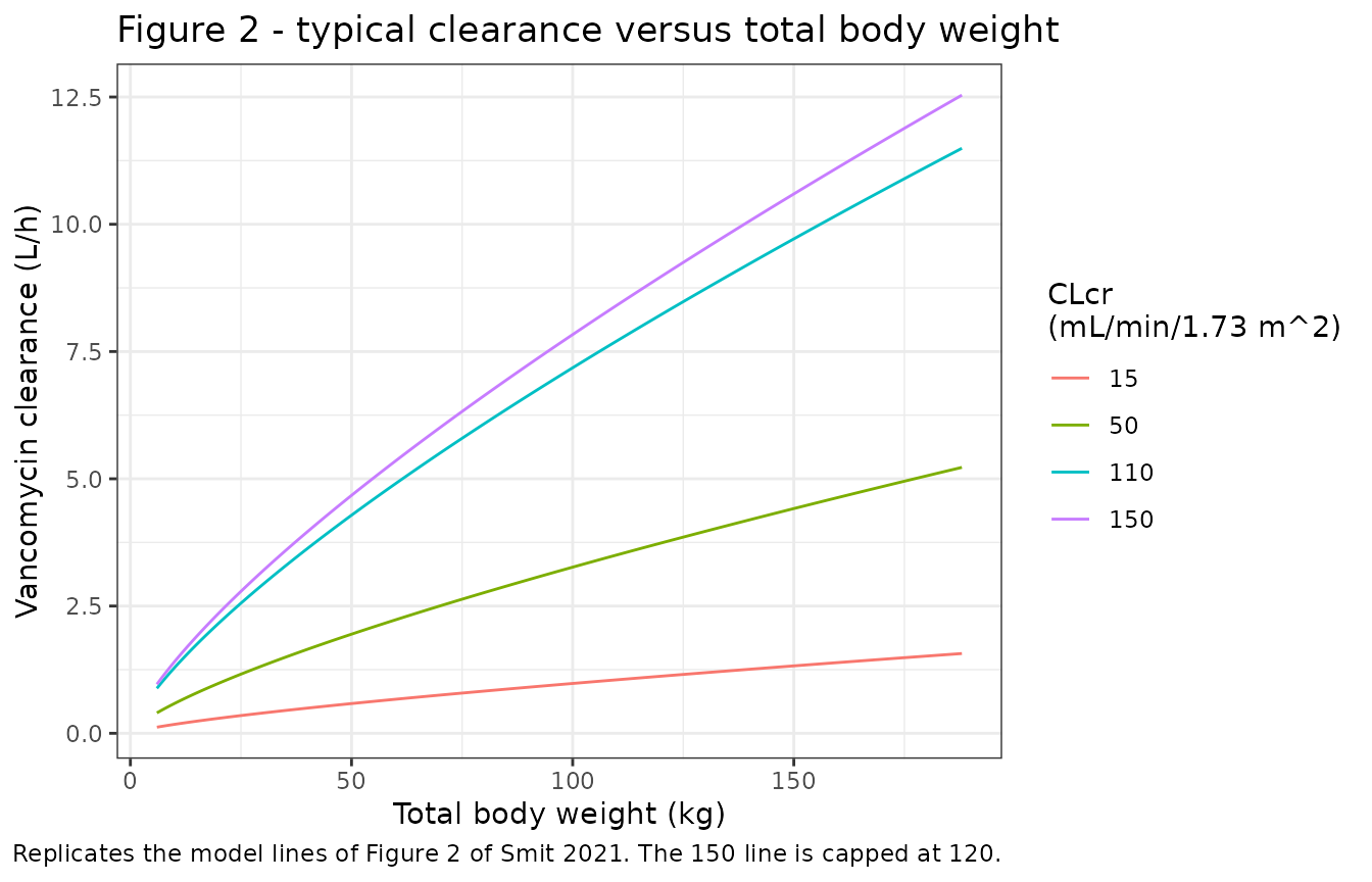

The paper plots the 150 mL/min/1.73 m^2 line even though the model caps CLcr at 120, so that line is the CLcr = 120 line: 1.2 times the typical clearance at CLcr 100.

Between-subject variability around the guideline

The paper’s Figure 4 deliberately omits between-subject variability. The stochastic simulation below shows how much it matters, for 200 virtual normal-weight 25 kg children with CLcr 120 mL/min/1.73 m^2 dosed 15 mg/kg every 6 hours.

rxode2::rxSetSeed(20210411)
n_sub <- 200
stoch_events <- lapply(seq_len(n_sub), function(i) {
  sc <- tibble::tibble(id = i, WT = 25, CRCL = 120, tau = 6, first_mgkg = 15, dose_mgkg = 15, scenario = "25 kg, CLcr 120")
  build_fig4_events(sc)
}) |>
  dplyr::bind_rows() |>
  dplyr::arrange(id, time, dplyr::desc(evid))
sim_stoch <- rxode2::rxSolve(mod, events = stoch_events, keep = "WT") |>
  as.data.frame()
#> ℹ parameter labels from comments will be replaced by 'label()'
auc3_stoch <- sim_stoch |>
  dplyr::group_by(id) |>
  dplyr::summarise(auc_day3 = auc_window(dplyr::pick(time, Cc), 48, 72), .groups = "drop")
typical_auc3 <- chk$auc_day3_sim[chk$scenario == "12 year - 25 kg - normal weight | CLcr 120"]
knitr::kable(
  tibble::tibble(
    Statistic = c("Typical-value AUCday3", "Median AUCday3", "5th percentile", "95th percentile", "Fraction within 400-700"),
    Value = c(
      typical_auc3, stats::median(auc3_stoch$auc_day3),
      stats::quantile(auc3_stoch$auc_day3, c(0.05, 0.95)),
      mean(auc3_stoch$auc_day3 >= 400 & auc3_stoch$auc_day3 <= 700)
    )
  ),
  digits = 2,
  caption = "AUCday3 (mg*h/L) with between-subject variability, 200 virtual subjects."
)

AUCday3 (mg*h/L) with between-subject variability, 200 virtual subjects.

Statistic	Value
Typical-value AUCday3	533.28
Median AUCday3	523.44
5th percentile	330.27
95th percentile	770.58
Fraction within 400-700	0.74

# Centre, not extremes: with log-normal IIV on CL, the median AUC tracks the
# typical-value AUC.
stopifnot(abs(stats::median(auc3_stoch$auc_day3) / typical_auc3 - 1) < 0.1)

With a 28.7% CV on clearance, a substantial fraction of individuals falls outside the 400-700 mg*h/L window even when the typical individual sits in the middle of it, which is why the paper recommends Bayesian forecasting on therapeutic drug monitoring samples to individualise exposure.

Assumptions and deviations

• Residual error scale. Table II prints the final proportional error as 0.0789 with the footnote “Proportional error is shown as sigma”. The maintainers read it as the NONMEM $SIGMA variance of the additive error on log-transformed concentrations, giving a log-scale SD of sqrt(0.0789) = 0.281. Three lines of evidence support this: the supplement control stream’s $SIGMA 0.0788 ; PROP ERR IN LOGDOMAIN is a variance by NONMEM definition and is essentially the published value; the reported 24% eta shrinkage on CL with a median of 4 samples per patient implies a residual variance near 0.08, whereas an SD of 0.0789 (variance 0.0062) would imply almost no CL shrinkage; and the reported 16% epsilon shrinkage is consistent with the same variance. The residual error does not affect the typical-value Figure 4 reproduction.
• Covariance of the CL and V2 random effects. Table II prints the covariance directly (-0.085, correlation about -0.34 with the variances above); it is used as printed.
• V2 variability. Table II gives 110% CV; the supplement Results give 109.5%. The table value is used (variance 0.793 vs 0.788).
• Random effects on V1 and Q are fixed to zero in the supplement control stream and are omitted from the model.
• Bedside Schwartz constant. Main-text Eq. 1 prints 0.41 while the supplement Results give 0.413. The model takes CLcr as an input, so the choice only matters when a user derives CRCL from height and creatinine.
• CLcr cap. The model applies the 120 mL/min/1.73 m^2 cap internally, so users supply the uncapped bedside Schwartz value.
• Figure 4 regimen details. Two details are not stated in the Methods but are needed to reproduce the Figure 4 AUCday1 labels; both are consistent with the paper and together make every one of the 72 labels reproduce. First, in Table III only the rows marked with footnote (a) (CLcr at or below 90) start with a 15 mg/kg first dose; the CLcr above 90 row has no footnote, so its first dose is the maintenance dose (18 mg/kg for patients over 70 kg). Second, doses are infused at 10 mg/min with a 60-min minimum, the usual vancomycin infusion-rate limit, so large doses run longer than 60 min. The regimen-sensitivity section above shows the simplified alternative misses the published AUCday1 by up to 8%.
• Cmin at day 3 is taken as the first trough after the 48 h dose. The published Cmin values run up to about 1.5% above the exact trough.
• No correction notice for the article was found as of 2026-09-28.