Hepatobiliary and renal clearance of [11C]AM7 and [11C]MT107 in mice (Taddio 2018)
Source:vignettes/articles/Taddio_2018_hepatobiliary_transport_pet_pbpk.Rmd
Taddio_2018_hepatobiliary_transport_pet_pbpk.RmdModel and source
- Citation: Taddio MF, Mu L, Keller C, Schibli R, Kramer SD. Physiologically Based Pharmacokinetic Modelling with Dynamic PET Data to Study the In Vivo Effects of Transporter Inhibition on Hepatobiliary Clearance in Mice. Contrast Media Mol Imaging. 2018;2018:5849047. doi:10.1155/2018/5849047. PMCID: PMC6008768. Model structure and compartment labels: Figure 2. Mass-transfer rate constants, peripheral-tissue volume and infusion duration: Supplementary Table 1, row ‘MT107 control / Average’ (n = 4). Derived clearance, extraction-ratio and tissue-distribution equations: Materials and Methods section 2.3, equations 2, 3 and 4. Organ volumes, blood volume, hematocrit, plasma flows and glomerular filtration rate: Materials and Methods sections 2.2 and 2.3, and the footer of Supplementary Table 1.
- Article: https://doi.org/10.1155/2018/5849047
- Supplement (Supplementary Figures 1-4 and Supplementary Table 1): https://doi.org/10.1155/2018/5849047 (Supplementary
Materials link on the article page; also available as
5849047.f1.pdfwith the open-access record, PMC6008768)
Taddio and colleagues repurposed dynamic whole-body mouse PET data
acquired with two investigational carbon-11 CD80 tracers and asked
whether the images alone carry enough information to fit a whole-body
compartmental (PBPK-style) model, and whether such a model can detect a
transporter-mediated drug-drug interaction in vivo. Tracer
amounts in blood plasma, liver, gallbladder plus intestines, kidneys and
peripheral tissue were read off volumes of interest and fitted jointly
to the compartment system of the paper’s Figure 2. The paper’s
scientific claim is the comparison of [11C]MT107 with and
without a prior dose of cyclosporine, an inhibitor of P-glycoprotein,
OATP1B1, OATP1B3 and BCRP.
The paper contributes three models to nlmixr2lib. The authors fitted every scan independently and estimated no drug-interaction coefficient, so the cyclosporine effect is carried by a separate parameter set rather than by a covariate.
model_names <- c(
  "Taddio_2018_am7_mouse_pbpk",
  "Taddio_2018_mt107_mouse_pbpk",
  "Taddio_2018_mt107_cyclosporine_mouse_pbpk"
)
uis <- lapply(model_names, function(n) rxode2::rxode(readModelDb(n)))
names(uis) <- model_names

tibble::tibble(
  Model = model_names,
  Tracer = c("[11C]AM7", "[11C]MT107", "[11C]MT107"),
  Condition = c("control (vehicle)", "control", "cyclosporine 50 mg/kg i.v."),
  `Source row` = c(
    "Suppl. Table 1, 'AM7 Control / Fig. 6A'",
    "Suppl. Table 1, 'MT107 control / Average' (n = 4)",
    "Suppl. Table 1, 'MT107 Ciclosporin / Average' (n = 4)"
  )
) |>
knitr::kable(caption = "Models contributed by Taddio 2018.")| Model | Tracer | Condition | Source row |
|---|---|---|---|
| Taddio_2018_am7_mouse_pbpk | [11C]AM7 | control (vehicle) | Suppl. Table 1, ‘AM7 Control / Fig. 6A’ |
| Taddio_2018_mt107_mouse_pbpk | [11C]MT107 | control | Suppl. Table 1, ‘MT107 control / Average’ (n = 4) |
| Taddio_2018_mt107_cyclosporine_mouse_pbpk | [11C]MT107 | cyclosporine 50 mg/kg i.v. | Suppl. Table 1, ‘MT107 Ciclosporin / Average’ (n = 4) |
Population
All scans were of 7-to-10-week-old female immunodeficient mice
(C.B.17 SCID for [11C]MT107, CD1 nude for
[11C]AM7) weighing 16.9 to 25.3 g and carrying
hCD80-positive Raji xenografts; the radioactivity fraction in the
xenografts was negligible and was not modelled. Tracer was injected
intravenously over about 10 s at 3 to 14 MBq and under 20 nmol/kg.
Cyclosporine 50 mg/kg was given intravenously 30 to 50 min before
tracer. Imaging started 60 s after injection and ran for 60 min, so
the first minute after injection is missing from every data
set - a limitation the authors call out explicitly, because
that window is the one that most constrains the plasma-to-tissue rate
constants.
Group sizes were n = 2 for [11C]AM7 control, n = 1 for
[11C]AM7 after cyclosporine (not modelled, see Errata), n =
4 for [11C]MT107 control and n = 4 for
[11C]MT107 after cyclosporine.
str(uis[["Taddio_2018_mt107_mouse_pbpk"]]$population)
#> List of 12
#>  $ species       : chr "mouse (female C.B.17 SCID, carrying hCD80-positive Raji xenografts)"
#>  $ n_subjects    : int 4
#>  $ n_studies     : int 1
#>  $ age_range     : chr "7-10 weeks"
#>  $ weight_range  : chr "16.9-22.4 g"
#>  $ weight_median : chr "18.95 g (mean of the four control scans)"
#>  $ sex_female_pct: num 100
#>  $ disease_state : chr "hCD80-positive Raji xenograft-bearing immunodeficient mice; the xenograft radioactivity fraction was negligible"| __truncated__
#>  $ dose_range    : chr "3-14 MBq [11C]MT107 (< 20 nmol/kg) as a ~10 s intravenous injection in 100-200 uL saline with 5% ethanol"
#>  $ regions       : chr "Switzerland (ETH Zurich)"
#>  $ co_medication : chr "none (three scans without vehicle, one with vehicle 13% ethanol 2 mL/kg 30 min before tracer)"
#>  $ notes         : chr "Data were repurposed from PET experiments that had not been designed for PBPK modelling. Scans were acquired on"| __truncated__
Model structure
All nine states hold a decay-corrected radioactivity amount, and every transfer is first-order with a rate constant in 1/min, so the model is linear and its derived quantities do not depend on the injected dose.
| Paper label (Figure 2) | nlmixr2lib state | Role |
|---|---|---|
| Blood plasma (B) | central |
dosing and sampling compartment |
| Liver 1 (H1) | liver_exchange |
hepatic pool exchanging reversibly with plasma |
| Liver 2 (H2) | liver_deep |
hepatic pool fed irreversibly from H1; source of biliary excretion |
| Gallbladder and intestines (G) | gallbladder_intestine |
combined biliary and intestinal lumen |
| Kidneys 1 (R1) | kidney_exchange |
renal pool exchanging with plasma; source of urinary excretion |
| Kidneys 2 (R2) | kidney_deep |
renal pool reachable only through R1 |
| Tissue 1 (T1) | peripheral1 |
fast peripheral pool |
| Tissue 2 (T2) | peripheral2 |
slow peripheral pool |
| Urinary bladder (U) | urine |
urinary excretion |
The authors note that fits were equally good with the two pools of an
organ arranged in parallel off plasma, so the serial arrangement is a
description of the time-activity curves rather than an anatomical claim.
The five organ sub-states are therefore declared as
paper_specific_compartments rather than introduced as new
canonical compartment names.
Two structural facts drive everything that follows. First, plasma
splits into the two peripheral pools at fbt1 * kbt and
(1 - fbt1) * kbt, so kbt is the
total plasma-to-tissue rate constant. Second,
gallbladder_intestine and urine have no exit
other than the slow intestinal reabsorption kgh1, because
the bladder was outside the field of view and there is no defecation
during a 60-minute scan; the system therefore conserves mass
exactly.
uis[["Taddio_2018_mt107_mouse_pbpk"]]$modelDesc
#> [1] "rxode2-based free-form 9-cmt ODE model"
Source trace
Every ini() entry carries an in-file comment pointing at
its source location. They are collected here for review.
| Equation / parameter | Source location |
|---|---|
Compartment system, all nine d/dt() lines |
Figure 2 (model diagram, including the arrow directions and the
fbt1 * kbt / (1 - fbt1) * kbt split) |
kbh1, kh1b, kh1h2,
kh2g, kgh1, kbg
|
Supplementary Table 1, columns kBH1, KH1B,
kH1H2, kH2G, kGH1,
kBG
|
kbr1, kr1b, kr1r2,
kr2r1, kr1u
|
Supplementary Table 1, columns kBR1, kR1B,
kR1R2, kR2R1, kR1U
|
kbt, kt1b, kt2b
|
Supplementary Table 1, columns kBT, kT1B,
kT2B
|
fbt1 |
Supplementary Table 1 column 1-fBT1, complemented (the
table reports the slow-pool fraction) |
vtissue_bw |
Supplementary Table 1 column VTissue/BW; estimated
during fitting (Methods 2.2) |
vplasma_bw = 0.03276 mL/g |
Supplementary Table 1 footer; Methods 2.3,
VBlood * (1 - hematocrit)
|
vliver_bw = 0.065 mL/g, vkidney_bw =
0.0164 mL/g |
Methods 2.2 (Davies and Morris) |
vblood_bw = 0.0585 mL/g, hct = 0.44 |
Methods 2.2 |
qh = 1000 uL/min, qr = 730 uL/min,
gfr = 160 uL/min |
Supplementary Table 1 footer; Methods 2.3; Results 3.2 |
clh (equation 2) |
Methods 2.3, equation 2 |
clr (equation 3) |
Methods 2.3, equation 3 |
dtissue (equation 4) |
Methods 2.3, equation 4 |
eh = clh / qh
|
Methods 2.3, “The extraction ratio EH for liver was estimated as ratio between CLH and QP,H” |
| Body weight and injected activity per scan | Supplementary Table 1 column BW; A(0) annotations
printed inside the Figure 6 and Figure 7 panels |
| Infusion duration T = 0.15 min | Supplementary Table 1 column T
|
The scan-level answer key
Supplementary Table 1 reports, for each of the eleven fitted scans, both the fitted rate constants and the derived quantities computed from them. That makes the supplement an exact answer key: every derived value must be recoverable from the rate constants in the same row. The table below transcribes it.
scans <- tibble::tribble(
  ~scan,           ~tracer,      ~arm,            ~bw_g, ~a0_kbq,
  "Fig. 6(a)",     "[11C]AM7",   "control",        24.4,   13870,
  "Fig. 6(b)",     "[11C]AM7",   "control",        19.7,    8230,
  "Suppl. Fig. 3", "[11C]AM7",   "cyclosporine",   25.3,   12500,
  "Fig. 7(a)",     "[11C]MT107", "control",        16.9,    6890,
  "Fig. 7(b)",     "[11C]MT107", "control",        18.1,    7020,
  "Fig. 7(c)",     "[11C]MT107", "control",        18.4,    5470,
  "Fig. 7(d)",     "[11C]MT107", "control",        22.4,    2970,
  "Fig. 7(e)",     "[11C]MT107", "cyclosporine",   19.3,    6580,
  "Fig. 7(f)",     "[11C]MT107", "cyclosporine",   21.2,    4850,
  "Fig. 7(g)",     "[11C]MT107", "cyclosporine",   21.0,   11650,
  "Fig. 7(h)",     "[11C]MT107", "cyclosporine",   19.1,   11710
) |>
  mutate(
    # Fitted mass-transfer rate constants (1/min), Supplementary Table 1
    kbh1  = c(.2595, .5099, .1757, .3825, .5365, .5769, 1.0984, 1.4079, 1.1645, .6413, 1.4933),
    kh1b  = c(.2306, .3992, .2414, .3087, .6660, .9420, 1.6095, 3.1816, 2.3960, 1.6058, 2.5142),
    kh1h2 = c(.1569, .2080, .0620, .0716, .0843, .0572, .0959, .0529, .0688, .0790, .0286),
    kh2g  = c(.0193, .0145, .0037, 1.9446, .1573, .0509, .1601, .0736, .1381, .2424, .1761),
    kgh1  = c(.0397, .0226, .0161, .0096, .0047, .0052, .0113, .0126, .0048, .0100, .0049),
    kbg   = c(.0236, .0107, .0093, 0, 0, 0, 0, 0, 0, 0, 0),
    kbr1  = c(.3819, .4691, .2939, .1178, .1185, .1108, .1654, .2000, .1610, .0874, .1821),
    kr1b  = c(.2497, .2939, .4502, .3626, .4322, .5968, .9025, 1.6135, .8661, .3313, .8860),
    kr1r2 = c(0, .0035, .1798, .0023, .0120, .0045, .0633, .1559, .0634, .0540, .0471),
    kr2r1 = c(.2676, .0655, .0459, .0002, .0642, .1438, .0003, .0806, .0243, .0107, .0759),
    kr1u  = c(.2796, .4241, .3665, .1172, .1318, .1009, .0424, .4096, .2080, .1526, .1194),
    kbt   = c(.8149, .4235, .5934, 1.7587, .5458, 1.1588, 1.0125, 1.8242, .7726, .3913, 2.1846),
    kt1b  = c(163.382, 110.3334, 146.4993, 2.3107, .7509, 3.6017, 2.3428, 4.78, .9772, .5014, 5.0072),
    one_minus_fbt1 = c(.3038, 1, 1, .0344, .1141, .0474, .0797, .0499, .1530, .2265, .0369),
    kt2b  = c(.1222, .1948, .1516, .0425, .0327, .0312, .0370, .0300, .0335, .0310, .0397),
    vtissue_bw = c(.6001, .6000, .7450, .7781, .6198, .7690, .8033, .6930, .9224, .7706, .7816),
    # Derived quantities printed in the same rows
    p_clh   = c(83.97, 112.742, 29.737, 39.853, 35.74, 19.915, 45.348, 14.546, 22.589, 20.681, 10.498),
    p_clbg  = c(18.826, 6.888, 7.69, 0, 0, 0, 0, 0, 0, 0, 0),
    p_clr   = c(161.258, 178.824, 109.306, 15.935, 16.427, 9.664, 5.445, 25.599, 21.657, 18.963, 13.536),
    p_cltot = c(264.054, 298.454, 146.732, 55.788, 52.167, 29.579, 50.793, 40.146, 44.246, 39.643, 24.034),
    p_eh      = c(.084, .113, .030, .040, .036, .020, .045, .015, .023, .021, .010),
    p_dtissue = c(.114, .119, .172, .091, .135, .088, .105, .161, .149, .147, .103),
    p_clr_gfr = c(1.008, 1.118, .683, .100, .103, .060, .034, .160, .135, .119, .085),
    # Biexponential plasma fit (equation 1) for the same scans
    b_v1 = c(3.0316, 2.2853, 4.1679, 1.4672, 1.5460, 1.2381, 1.6977, 1.2217, 1.4899, 1.3982, 1.4007),
    b_vz = c(10.3465, 9.3597, 8.0049, 2.9144, 2.7537, 1.9231, 3.0572, 4.1050, 3.7155, 3.2283, 2.2637),
    b_l1 = c(.1963, .2955, .2044, .1156, .1102, .1345, .1244, .1222, .1589, .1558, .1210),
    b_lz = c(.0234, .0271, .0206, .0217, .0204, .0198, .0220, .0089, .0151, .0159, .0161),
    b_cl = c(241.854, 253.191, 164.996, 63.178, 56.041, 37.989, 67.370, 36.526, 56.088, 51.185, 36.363),
    # Model inputs
    fbt1 = 1 - one_minus_fbt1,
    WT = bw_g / 1000,
    id = row_number(),
    # A(0) is printed inside the Figure 6 / Figure 7 panels. The Suppl. Fig. 3
    # scan has no panel annotation, but it is the scan of Figure 3(b), whose
    # caption gives 12.5 MBq; that is the value used here.
    a0_mbq = a0_kbq / 1000,
    group = paste(tracer, arm)
  )

knitr::kable(
  scans |> select(scan, tracer, arm, `BW (g)` = bw_g, `A(0) (kBq)` = a0_kbq),
  caption = "The eleven fitted scans (Supplementary Table 1; A(0) from the Figure 6 / Figure 7 panel annotations)."
)| scan | tracer | arm | BW (g) | A(0) (kBq) |
|---|---|---|---|---|
| Fig. 6(a) | [11C]AM7 | control | 24.4 | 13870 |
| Fig. 6(b) | [11C]AM7 | control | 19.7 | 8230 |
| Suppl. Fig. 3 | [11C]AM7 | cyclosporine | 25.3 | 12500 |
| Fig. 7(a) | [11C]MT107 | control | 16.9 | 6890 |
| Fig. 7(b) | [11C]MT107 | control | 18.1 | 7020 |
| Fig. 7(c) | [11C]MT107 | control | 18.4 | 5470 |
| Fig. 7(d) | [11C]MT107 | control | 22.4 | 2970 |
| Fig. 7(e) | [11C]MT107 | cyclosporine | 19.3 | 6580 |
| Fig. 7(f) | [11C]MT107 | cyclosporine | 21.2 | 4850 |
| Fig. 7(g) | [11C]MT107 | cyclosporine | 21.0 | 11650 |
| Fig. 7(h) | [11C]MT107 | cyclosporine | 19.1 | 11710 |
The body weights printed inside the Figure 6 and Figure 7 panels
agree with the BW column of Supplementary Table 1 for all
eleven scans, which confirms the row-to-panel mapping used throughout
this vignette.
Simulation
The mass-transfer rate constants and vtissue_bw are
supplied as per-subject columns, so a single rxSolve() call
reproduces all eleven scans. T = 0.15 min is the infusion
duration the fits used, entered as rate = amt / 0.15.
T_INF <- 0.15 # min; Supplementary Table 1 column 'T'

par_cols <- c(
  "kbh1", "kh1b", "kh1h2", "kh2g", "kgh1", "kbg",
  "kbr1", "kr1b", "kr1r2", "kr2r1", "kr1u",
  "kbt", "kt1b", "fbt1", "kt2b", "vtissue_bw"
)

obs_times <- sort(unique(c(seq(0, 68, by = 0.1), 1, 60, 68)))

events <- bind_rows(lapply(seq_len(nrow(scans)), function(i) {
  bind_rows(
    data.frame(
      id = scans$id[i], time = 0, amt = scans$a0_mbq[i],
      rate = scans$a0_mbq[i] / T_INF, evid = 1L, cmt = "central"
    ),
    data.frame(
      id = scans$id[i], time = obs_times, amt = NA_real_,
      rate = NA_real_, evid = 0L, cmt = "central"
    )
  )
})) |>
  left_join(scans[, c("id", "WT", "group", "scan", par_cols)], by = "id")

stopifnot(!anyDuplicated(unique(events[, c("id", "time", "evid")])))

# The AM7 model is used as the simulation engine because it is the one whose
# kbg and kr1r2 are free rather than fixed at zero; model() is byte-identical
# across the three files, and the per-scan parameter columns above override
# every ini() value, so the choice cannot affect any result.
sim <- rxode2::rxSolve(
  readModelDb("Taddio_2018_am7_mouse_pbpk"),
  events = events,
  keep = c("WT", "group", "scan"),
  atol = 1e-12, rtol = 1e-10
) |>
  as.data.frame()
#> Warning: multi-subject simulation without without 'omega'

per_scan <- sim |>
  group_by(id, scan, group) |>
  slice(1) |>
  ungroup() |>
  arrange(id)
Validation 1 - the derived clearances reproduce Supplementary Table 1
clh, clr, dtissue and
eh are the paper’s equations 2, 3 and 4 encoded in
model(). Recomputing them from each scan’s own rate
constants must return the values printed in the same row. This checks
the transcription of every rate constant and of the three equations, for
all eleven scans at once.
pct <- function(a, b) 100 * (a / b - 1)

derived <- scans |>
  select(scan, group, starts_with("p_")) |>
  bind_cols(per_scan |> select(clh, clbg, clr, cltot, eh, dtissue, clr_gfr)) |>
  mutate(
    `CLH (%)` = pct(clh, p_clh),
    `CLR (%)` = pct(clr, p_clr),
    `CL total (%)` = pct(cltot, p_cltot),
    `DTissue (%)` = pct(dtissue, p_dtissue),
    `CLR/GFR (%)` = pct(clr_gfr, p_clr_gfr),
    `EH (absolute)` = eh - p_eh,
    `CL BG (uL/min)` = clbg - p_clbg
  )

derived |>
  select(Scan = scan, `CLH (%)`, `CLR (%)`, `CL total (%)`,
         `DTissue (%)`, `CLR/GFR (%)`, `EH (absolute)`) |>
  knitr::kable(
    digits = c(0, 2, 2, 2, 2, 2, 5),
    caption = "Model minus Supplementary Table 1, as a percentage (EH as an absolute difference because it is printed to only three decimals)."
)| Scan | CLH (%) | CLR (%) | CL total (%) | DTissue (%) | CLR/GFR (%) | EH (absolute) |
|---|---|---|---|---|---|---|
| Fig. 6(a) | 0.02 | 0.00 | 0.02 | -2.82 | -0.01 | -0.00001 |
| Fig. 6(b) | -0.01 | 0.00 | 0.00 | -0.25 | -0.03 | -0.00027 |
| Suppl. Fig. 3 | 0.07 | 0.01 | 0.03 | 0.07 | 0.03 | -0.00024 |
| Fig. 7(a) | 0.04 | -0.03 | 0.02 | -0.14 | -0.43 | -0.00013 |
| Fig. 7(b) | 0.01 | -0.04 | -0.01 | -0.22 | -0.36 | -0.00026 |
| Fig. 7(c) | -0.04 | -0.05 | -0.04 | 0.06 | 0.61 | -0.00009 |
| Fig. 7(d) | -0.05 | 0.03 | -0.04 | 0.16 | 0.12 | 0.00033 |
| Fig. 7(e) | 0.09 | 0.01 | 0.04 | -0.26 | 0.01 | -0.00044 |
| Fig. 7(f) | -0.06 | -0.02 | -0.04 | 0.07 | 0.25 | -0.00043 |
| Fig. 7(g) | 0.03 | -0.01 | 0.01 | 0.14 | -0.41 | -0.00031 |
| Fig. 7(h) | 0.11 | -0.03 | 0.03 | -0.27 | -0.50 | 0.00051 |
# Deterministic arithmetic on printed values - no simulated cohort is involved,
# so these bounds are tightened to the accuracy actually achieved rather than
# padded for run-to-run noise. Realised maxima: 0.11 % on CLH, 0.05 % on CLR,
# 0.04 % on CL total, 0.61 % on CLR/GFR (the last is limited by CLR/GFR being
# printed to three decimals, e.g. 0.060 for a value of 0.0604).
stopifnot(
  max(abs(derived$`CLH (%)`)) < 0.5,
  max(abs(derived$`CLR (%)`)) < 0.5,
  max(abs(derived$`CL total (%)`)) < 0.5,
  max(abs(derived$`CLR/GFR (%)`)) < 1,
  # EH is printed to three decimals, so half of the last digit is 0.0005.
  max(abs(derived$`EH (absolute)`)) < 0.001,
  # CL BG is exactly zero for every [11C]MT107 scan and matches the printed
  # value for the three [11C]AM7 scans.
  max(abs(derived$`CL BG (uL/min)`)) < 0.05
)

# DTissue: ten of eleven scans agree to better than 0.3 %. The Figure 6(a) row
# is a documented internal inconsistency in the source and is excluded from the
# gate rather than the gate being widened to absorb it - see Errata.
dtissue_ok <- derived |> filter(scan != "Fig. 6(a)")
stopifnot(max(abs(dtissue_ok$`DTissue (%)`)) < 0.5)

sprintf(
  "DTissue, Fig. 6(a): model %.4f vs printed %.3f (%.2f %%) - documented source inconsistency",
  derived$dtissue[derived$scan == "Fig. 6(a)"],
  derived$p_dtissue[derived$scan == "Fig. 6(a)"],
  derived$`DTissue (%)`[derived$scan == "Fig. 6(a)"]
)
#> [1] "DTissue, Fig. 6(a): model 0.1108 vs printed 0.114 (-2.82 %) - documented source inconsistency"
Validation 2 - mass conservation
gallbladder_intestine and urine are
terminal within the scan, and no other route leaves the system, so the
nine states must sum to the injected activity at every time after the
infusion ends. This is the strongest available check on the ODE wiring:
any mis-signed or mis-paired transfer term breaks it immediately.
states <- c(
  "central", "liver_exchange", "liver_deep", "gallbladder_intestine",
  "kidney_exchange", "kidney_deep", "peripheral1", "peripheral2", "urine"
)

mass <- sim |>
  filter(time >= T_INF) |>
  mutate(total = rowSums(across(all_of(states)))) |>
  left_join(scans[, c("id", "a0_mbq")], by = "id") |>
  mutate(rel = abs(total / a0_mbq - 1))

sprintf("Worst relative mass-balance error over all scans and times: %.2e",
        max(mass$rel))
#> [1] "Worst relative mass-balance error over all scans and times: 3.33e-15"

# Solver tolerance, not model error: atol = 1e-12 / rtol = 1e-10 above.
stopifnot(max(mass$rel) < 1e-8)
Validation 3 - the ODEs reproduce the closed-form clearance equations
Equations 2 and 3 are steady-state expressions. Equation 2 is the
flux into bile divided by the plasma concentration once the hepatic
sub-system has equilibrated (the intestinal return kgh1 is
ignored in its derivation), and equation 3 is the flux into urine
divided by the plasma concentration, with the R1/R2 exchange cancelling
out because it is a closed loop. Driving the model with a constant
infusion and measuring those fluxes therefore tests the ODE wiring
against the paper’s own printed algebra - a check that the equation-2/3
evaluation inside model() cannot satisfy on its own.
# tmax must be long enough for the SLOWEST scan to converge, not the typical
# one. At tmax = 5000 min two scans are still short of steady state and miss
# the machine-precision gate below: the Suppl. Fig. 3 hepatic arm (kH2G =
# 0.0037 /min) by 1.7e-8 and the Fig. 7(d) renal arm (kR1U = 0.0424 /min with
# a large DTissue * VTissue reservoir) by 1.3e-7. At 50000 min every scan
# reaches machine precision, and the solve still costs well under a second
# because only two output rows are requested.
steady_state <- function(ui, pars, wt, tmax = 50000) {
  ev <- bind_rows(
    data.frame(time = 0, amt = 10 * tmax, rate = 1, evid = 1L, cmt = "central"),
    data.frame(time = tmax, amt = NA_real_, rate = NA_real_, evid = 0L, cmt = "central")
  )
  ev <- cbind(ev, as.data.frame(pars), WT = wt)
  tail(
    rxode2::rxSolve(ui, ev, returnType = "data.frame", atol = 1e-12, rtol = 1e-10),
    1
  )
}

mod_am7 <- readModelDb("Taddio_2018_am7_mouse_pbpk")

identity_check <- bind_rows(lapply(seq_len(nrow(scans)), function(i) {
  pars <- as.list(scans[i, par_cols])
  wt <- scans$WT[i]

  # Hepatic: switch off renal uptake and the intestinal return so plasma reaches
  # a true steady state and bile is the only sink.
  ph <- modifyList(pars, list(kbr1 = 0, kgh1 = 0))
  lh <- steady_state(mod_am7, ph, wt)

  # Renal: switch off hepatic uptake and the transintestinal route. The R1/R2
  # loop is decoupled as well, which is the paper's own simplification
  # ("compartments R1 and R2 were treated as one compartment") and does not
  # change equation 3.
  pr <- modifyList(pars, list(kbh1 = 0, kbg = 0, kr1r2 = 0, kr2r1 = 0))
  lr <- steady_state(mod_am7, pr, wt)

  tibble::tibble(
    scan = scans$scan[i],
    clh_ode = pars$kh2g * lh$liver_deep / lh$Cc * 1000,
    clh_eq2 = lh$clh,
    clr_ode = pars$kr1u * lr$kidney_exchange / lr$Cc * 1000,
    clr_eq3 = lr$clr
  )
})) |>
  mutate(
    hepatic_rel = abs(clh_ode / clh_eq2 - 1),
    renal_rel = abs(clr_ode / clr_eq3 - 1)
  )

sprintf(
  "Worst relative disagreement: hepatic %.2e, renal %.2e (machine precision)",
  max(identity_check$hepatic_rel), max(identity_check$renal_rel)
)
#> [1] "Worst relative disagreement: hepatic 4.30e-14, renal 2.22e-16 (machine precision)"
stopifnot(
  max(identity_check$hepatic_rel) < 1e-8,
  max(identity_check$renal_rel) < 1e-8
)
A second consequence of the structure is that the R2-to-R1 amount
ratio must converge to kr1r2 / kr2r1. Checking it on the
scan with the fastest renal exchange confirms the
kidney_exchange / kidney_deep wiring, which
the equation-3 gate above deliberately bypasses.
# Pick the scan whose R1/R2 loop equilibrates fastest AND is identifiable, i.e.
# the one maximising the SMALLER of the two rate constants. Selecting on kr2r1
# alone would land on Fig. 6(a), whose kr1r2 is 0, making the expected ratio
# 0 / 0.2676 = 0 and the relative check 0/0 = NaN.
i <- which.max(pmin(scans$kr1r2, scans$kr2r1))
pars <- modifyList(as.list(scans[i, par_cols]), list(kbh1 = 0, kbg = 0))
ss <- steady_state(mod_am7, pars, scans$WT[i])
observed_ratio <- ss$kidney_deep / ss$kidney_exchange
expected_ratio <- scans$kr1r2[i] / scans$kr2r1[i]
sprintf("%s: R2/R1 = %.5f, kr1r2/kr2r1 = %.5f", scans$scan[i], observed_ratio, expected_ratio)
#> [1] "Fig. 7(e): R2/R1 = 1.93424, kr1r2/kr2r1 = 1.93424"
stopifnot(abs(observed_ratio / expected_ratio - 1) < 1e-4)
Validation 4 - the cyclosporine effect reported in Table 1
Table 1 summarises the group means. Reproducing them from the
per-scan model outputs checks that the two [11C]MT107 model
files carry the right arm.
group_summary <- per_scan |>
  filter(group != "[11C]AM7 cyclosporine") |>
  group_by(group) |>
  summarise(
    CLH = mean(clh), CLH_sd = sd(clh),
    CLR = mean(clr), CLR_sd = sd(clr),
    EH = mean(eh),
    CLtot = mean(cltot),
    `CLH/CLR` = mean(clh / clr),
    .groups = "drop"
  )

published_table1 <- tibble::tribble(
  ~group,                    ~p_CLH,  ~p_CLR, ~p_EH,  ~p_CLtot, ~`p_CLH/CLR`,
  "[11C]MT107 control",       35.2,    11.9,  0.035,   47.1,     3.8,
  "[11C]MT107 cyclosporine",  17.1,    19.9,  0.017,   37.0,     0.9
)

cmp_t1 <- group_summary |>
  inner_join(published_table1, by = "group")

cmp_t1 |>
  transmute(
    Group = group,
    `CLH model` = CLH, `CLH Table 1` = p_CLH,
    `CLR model` = CLR, `CLR Table 1` = p_CLR,
    `EH model` = EH, `EH Table 1` = p_EH,
    `CLH/CLR model` = `CLH/CLR`, `CLH/CLR Table 1` = `p_CLH/CLR`
  ) |>
knitr::kable(digits = 3, caption = "Group means from the model versus Table 1.")| Group | CLH model | CLH Table 1 | CLR model | CLR Table 1 | EH model | EH Table 1 | CLH/CLR model | CLH/CLR Table 1 |
|---|---|---|---|---|---|---|---|---|
| [11C]MT107 control | 35.211 | 35.2 | 11.864 | 11.9 | 0.035 | 0.035 | 3.766 | 3.8 |
| [11C]MT107 cyclosporine | 17.083 | 17.1 | 19.937 | 19.9 | 0.017 | 0.017 | 0.870 | 0.9 |
# Table 1 rounds to three significant figures, so these are exact reproductions
# to within the printed precision, not approximations.
stopifnot(
  max(abs(cmp_t1$CLH / cmp_t1$p_CLH - 1)) < 0.01,
  max(abs(cmp_t1$CLR / cmp_t1$p_CLR - 1)) < 0.01,
  max(abs(cmp_t1$CLtot / cmp_t1$p_CLtot - 1)) < 0.01,
  max(abs(cmp_t1$EH - cmp_t1$p_EH)) < 0.0005,
  # CLH/CLR is printed to ONE decimal, so it is gated on an absolute difference
  # of half the last digit rather than on a percentage. A relative bound is the
  # wrong instrument here: the cyclosporine mean is 0.8695 against a printed
  # 0.9, an exact reproduction that nonetheless looks like a 3.4 % miss.
  max(abs(cmp_t1$`CLH/CLR` - cmp_t1$`p_CLH/CLR`)) < 0.05
)

# Results 3.3: "CLH and EH of [11C]MT107 were significantly reduced to 48% of
# the respective values in the absence of cyclosporine".
ratio_clh <- cmp_t1$CLH[cmp_t1$group == "[11C]MT107 cyclosporine"] /
  cmp_t1$CLH[cmp_t1$group == "[11C]MT107 control"]
sprintf("CLH after cyclosporine, as a fraction of control: %.3f (paper: 0.48)", ratio_clh)
#> [1] "CLH after cyclosporine, as a fraction of control: 0.485 (paper: 0.48)"
stopifnot(abs(ratio_clh - 0.48) < 0.02)

# Results 3.3: "CLR of [11C]MT107 was increased 1.7-fold on average".
ratio_clr <- cmp_t1$CLR[cmp_t1$group == "[11C]MT107 cyclosporine"] /
  cmp_t1$CLR[cmp_t1$group == "[11C]MT107 control"]
sprintf("CLR after cyclosporine, as a fold change: %.2f (paper: 1.7)", ratio_clr)
#> [1] "CLR after cyclosporine, as a fold change: 1.68 (paper: 1.7)"
stopifnot(abs(ratio_clr - 1.7) < 0.1)
The three model files are also checked against their own designated
rows, using the default ini() values rather than the
per-scan overrides above.
default_row <- function(name, wt, a0) {
  ev <- bind_rows(
    data.frame(time = 0, amt = a0, rate = a0 / T_INF, evid = 1L, cmt = "central"),
    data.frame(time = 1, amt = NA_real_, rate = NA_real_, evid = 0L, cmt = "central")
  )
  ev$WT <- wt
  s <- rxode2::rxSolve(readModelDb(name), ev, returnType = "data.frame",
                       atol = 1e-12, rtol = 1e-10)
  s[1, c("clh", "clbg", "clr", "cltot", "eh", "dtissue")]
}

defaults <- bind_rows(
  default_row("Taddio_2018_am7_mouse_pbpk", 0.0244, 13.87),
  default_row("Taddio_2018_mt107_mouse_pbpk", 0.01895, 10),
  default_row("Taddio_2018_mt107_cyclosporine_mouse_pbpk", 0.02015, 10)
) |>
  mutate(Model = model_names, .before = 1)

knitr::kable(defaults, digits = 4,
caption = "Derived quantities at each model file's default ini() values.")| Model | clh | clbg | clr | cltot | eh | dtissue |
|---|---|---|---|---|---|---|
| Taddio_2018_am7_mouse_pbpk | 83.9890 | 18.8645 | 161.2570 | 264.1105 | 0.0840 | 0.1108 |
| Taddio_2018_mt107_mouse_pbpk | 32.4625 | 0.0000 | 11.6161 | 44.0786 | 0.0325 | 0.1152 |
| Taddio_2018_mt107_cyclosporine_mouse_pbpk | 17.9345 | 0.0000 | 20.1789 | 38.1135 | 0.0179 | 0.2030 |
# The AM7 file carries a single scan, so it must match Fig. 6(a) exactly.
stopifnot(abs(defaults$clh[1] / 83.97 - 1) < 0.005,
          abs(defaults$clr[1] / 161.258 - 1) < 0.005,
          abs(defaults$clbg[1] / 18.826 - 1) < 0.005)

# The two MT107 files carry the MEAN rate constants. Equation 2 is a non-linear
# function of them, so evaluating it at the mean parameters is NOT the mean of
# the per-scan values; the gap is a property of the averaging, not an error.
sprintf(
  "MT107 control: CLH at the mean rate constants = %.1f uL/min; mean of the four per-scan CLH = %.1f uL/min (%.1f %%)",
  defaults$clh[2], cmp_t1$CLH[cmp_t1$group == "[11C]MT107 control"],
  pct(defaults$clh[2], cmp_t1$CLH[cmp_t1$group == "[11C]MT107 control"])
)
#> [1] "MT107 control: CLH at the mean rate constants = 32.5 uL/min; mean of the four per-scan CLH = 35.2 uL/min (-7.8 %)"
stopifnot(abs(pct(defaults$clh[2], 35.214)) < 12,
          abs(pct(defaults$clh[3], 17.078)) < 15)
Replicate published figures
tidy_curves <- function(df) {
  # No evid filter: rxSolve() returns observation records only (addDosing is
  # FALSE by default) and its output carries no evid column at all, so
  # filtering on one errors rather than being a harmless no-op.
  df |>
    transmute(
      time, scan, group,
      Plasma = central, Liver = Aliver, `Bile & intestines` = Agallbladder,
      Kidneys = Akidney, Tissue = Atissue, Urine = Aurine
    ) |>
    pivot_longer(Plasma:Urine, names_to = "Region", values_to = "kBq") |>
    mutate(kBq = kBq * 1000)
}

curves <- tidy_curves(sim)

curves |>
  filter(scan == "Fig. 6(a)") |>
  ggplot(aes(time, kBq, colour = Region)) +
  geom_line(linewidth = 0.8) +
  labs(
    x = "Time (min)", y = "Radioactivity (kBq)",
    title = "[11C]AM7, control, 13,870 kBq, 24.4 g",
    caption = "Replicates Figure 6(a) of Taddio 2018. The urine curve was PREDICTED, not fitted."
  ) +
  theme_bw()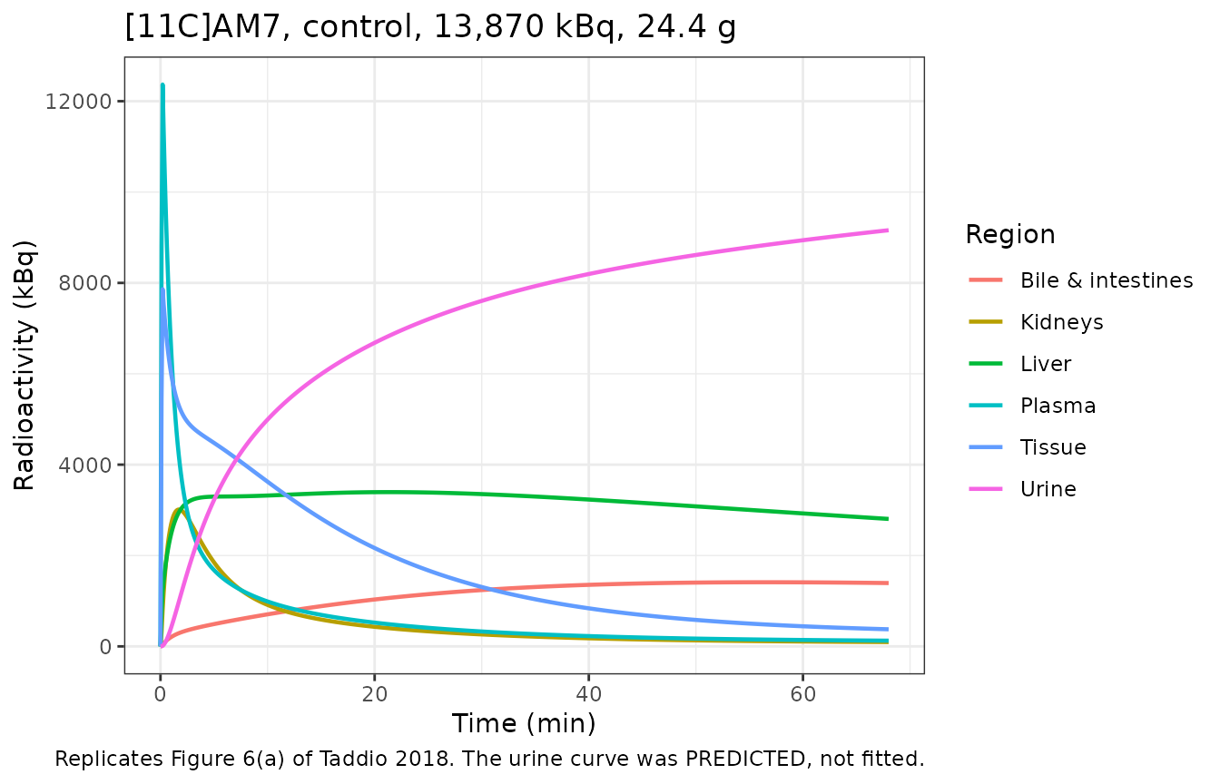
Replicates Figure 6(a) of Taddio 2018.
Figure 6(a) is the paper’s own validation scan: the urinary bladder was inside the field of view and the image-derived urine curve was deliberately withheld from the objective function, so the modelled urine curve is a prediction. The published panel reaches roughly 9,000 kBq of urinary activity at 60 min, with liver near 3,000 kBq and bile plus intestines near 1,300 kBq.
at60 <- sim |> filter(scan == "Fig. 6(a)", abs(time - 60) < 1e-6) |> slice(1)
tibble::tibble(
  Region = c("Urine", "Liver", "Bile & intestines"),
  `Model (kBq)` = c(at60$Aurine, at60$Aliver, at60$Agallbladder) * 1000,
  `Figure 6(a), read off the panel (kBq)` = c(9000, 3000, 1300)
) |>
knitr::kable(digits = 0, caption = "Model versus the published Figure 6(a) panel at 60 min.")| Region | Model (kBq) | Figure 6(a), read off the panel (kBq) |
|---|---|---|
| Urine | 8940 | 9000 |
| Liver | 2926 | 3000 |
| Bile & intestines | 1410 | 1300 |
# Bounds are generous because the reference values are read off a printed plot,
# not tabulated. They still go red on any gross structural or unit error, which
# would move these by multiples rather than by percent.
stopifnot(
  abs(at60$Aurine * 1000 / 9000 - 1) < 0.15,
  abs(at60$Aliver * 1000 / 3000 - 1) < 0.15,
  abs(at60$Agallbladder * 1000 / 1300 - 1) < 0.25
)
curves |>
  filter(grepl("Fig. 7", scan)) |>
  ggplot(aes(time, kBq, colour = Region)) +
  geom_line(linewidth = 0.7) +
  facet_wrap(~scan, scales = "free_y", ncol = 4) +
  labs(
    x = "Time (min)", y = "Radioactivity (kBq)",
    title = "[11C]MT107: control (a-d, top row) and after cyclosporine (e-h, bottom row)",
    caption = "Replicates Figure 7 of Taddio 2018."
  ) +
  theme_bw() +
  theme(legend.position = "bottom")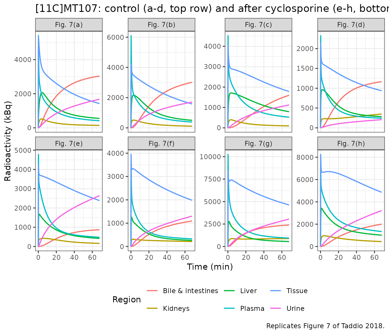
Replicates Figure 7 of Taddio 2018.
The qualitative claim of Results 3.3 is visible in the panels: under control conditions the combined gallbladder-and-intestine curve exceeds the modelled urine curve, whereas after cyclosporine it does not.
split_60 <- sim |>
  filter(grepl("Fig. 7", scan), abs(time - 60) < 1e-6) |>
  transmute(scan, group, biliary_over_urinary = Agallbladder / Aurine)

knitr::kable(split_60, digits = 2,
caption = "Biliary over urinary activity at 60 min, per scan.")| scan | group | biliary_over_urinary |
|---|---|---|
| Fig. 7(a) | [11C]MT107 control | 1.88 |
| Fig. 7(b) | [11C]MT107 control | 1.80 |
| Fig. 7(c) | [11C]MT107 control | 1.40 |
| Fig. 7(d) | [11C]MT107 control | 5.88 |
| Fig. 7(e) | [11C]MT107 cyclosporine | 0.34 |
| Fig. 7(f) | [11C]MT107 cyclosporine | 0.86 |
| Fig. 7(g) | [11C]MT107 cyclosporine | 0.82 |
| Fig. 7(h) | [11C]MT107 cyclosporine | 0.63 |
# The claim is directional and about the GROUP, so it is asserted on the group
# means rather than scan by scan.
means <- split_60 |> group_by(group) |> summarise(m = mean(biliary_over_urinary))
stopifnot(
  means$m[means$group == "[11C]MT107 control"] > 1,
  means$m[means$group == "[11C]MT107 cyclosporine"] <
    means$m[means$group == "[11C]MT107 control"]
)
PKNCA validation
The plasma curve is characterised with PKNCA over the paper’s
60-minute scan window. The reference is the paper’s own
alternative description of the same plasma data: the biexponential
infusion function of equation 1, evaluated with the per-scan
V1, Vz, lambda1 and
lambdaz of Supplementary Table 1 and put through the
identical PKNCA pipeline. Comparing the two is therefore a like-for-like
comparison of two published fits, not a comparison of a model against a
differently-computed summary.
# Equation 1 of Taddio 2018: biexponential response to a constant infusion of
# duration T.
biexp <- function(t, a0, tinf, v1, vz, l1, lz) {
  ramp <- pmin(t, tinf)
  decay <- pmax(t - tinf, 0)
  a0 / (tinf * v1) *
    ((l1 * v1 / vz - l1) / (l1 * (lz - l1)) * (1 - exp(-l1 * ramp)) * exp(-l1 * decay) +
      (l1 * v1 / vz - lz) / (lz * (l1 - lz)) * (1 - exp(-lz * ramp)) * exp(-lz * decay))
}

sim_nca <- sim |>
  filter(!is.na(Cc)) |>
  select(id, time, Cc, group) |>
  left_join(scans[, c("id", "a0_mbq", "b_v1", "b_vz", "b_l1", "b_lz")], by = "id") |>
  mutate(Cc_ref = biexp(time, a0_mbq, T_INF, b_v1, b_vz, b_l1, b_lz)) |>
  mutate(Cc_ref = ifelse(time == 0, 0, Cc_ref))

run_nca <- function(df, conc_col) {
  d <- df |>
    transmute(id, time, group, Cc = .data[[conc_col]]) |>
    filter(!is.na(Cc)) |>
    arrange(id, time)
  dose_df <- scans |> transmute(id, time = 0, amt = a0_mbq, group)
  PKNCA::pk.nca(PKNCA::PKNCAdata(
    PKNCA::PKNCAconc(d, Cc ~ time | group + id),
    PKNCA::PKNCAdose(dose_df, amt ~ time | group + id),
    intervals = data.frame(
      start = 0, end = 60,
      cmax = TRUE, tmax = TRUE, auclast = TRUE, half.life = TRUE
    )
  ))
}

nca_model <- run_nca(sim_nca, "Cc")
nca_ref <- run_nca(sim_nca, "Cc_ref")
Comparison against the published biexponential characterisation
ref_wide <- as.data.frame(nca_ref) |>
  filter(!is.na(PPORRES)) |>
  group_by(group, PPTESTCD) |>
  summarise(value = median(PPORRES), .groups = "drop") |>
  pivot_wider(names_from = PPTESTCD, values_from = value)

# Restrict to the four requested parameters. Asking PKNCA for half.life also
# returns its regression diagnostics (span.ratio, lambda.z n points, r.squared,
# clast.pred, ...). Those are properties of the 0.1-min simulation grid, not of
# the model, and comparing them star-flags rows that carry no pharmacological
# meaning - so they are excluded rather than left to clutter the table.
cmp <- nlmixr2lib::ncaComparisonTable(
  simulated = nca_model,
  reference = ref_wide,
  by = "group",
  params = c("cmax", "tmax", "auclast", "half.life"),
  units = c(cmax = "MBq/mL", auclast = "MBq*min/mL",
            tmax = "min", half.life = "min"),
  tolerance_pct = 20
)

knitr::kable(
  cmp,
  caption = "Compartment model versus the paper's own biexponential fit of the same plasma data (equation 1). * differs by more than 20%."
)| NCA parameter | group | Reference | Simulated | % diff |
|---|---|---|---|---|
| Cmax (MBq/mL) | [11C]AM7 control | 3.99 | 13.1 | +228.8%* |
| Cmax (MBq/mL) | [11C]AM7 cyclosporine | 2.96 | 13.2 | +347.8%* |
| Cmax (MBq/mL) | [11C]MT107 control | 4.44 | 8.62 | +94.0%* |
| Cmax (MBq/mL) | [11C]MT107 cyclosporine | 6.77 | 10.3 | +52.1%* |
| Tmax (min) | [11C]AM7 control | 0.2 | 0.2 | +0.0% |
| Tmax (min) | [11C]AM7 cyclosporine | 0.2 | 0.2 | +0.0% |
| Tmax (min) | [11C]MT107 control | 0.2 | 0.2 | +0.0% |
| Tmax (min) | [11C]MT107 cyclosporine | 0.2 | 0.2 | +0.0% |
| AUClast (MBq*min/mL) | [11C]AM7 control | 37.9 | 42.2 | +11.4% |
| AUClast (MBq*min/mL) | [11C]AM7 cyclosporine | 56 | 68.7 | +22.7%* |
| AUClast (MBq*min/mL) | [11C]MT107 control | 90.3 | 100 | +11.2% |
| AUClast (MBq*min/mL) | [11C]MT107 cyclosporine | 123 | 131 | +6.5% |
| t½ (min) | [11C]AM7 control | 27.2 | 56.3 | +106.9%* |
| t½ (min) | [11C]AM7 cyclosporine | 33.2 | 30.9 | -7.1% |
| t½ (min) | [11C]MT107 control | 31.3 | 67.5 | +115.8%* |
| t½ (min) | [11C]MT107 cyclosporine | 43.7 | 93.6 | +114.1%* |
The starred rows are expected and are discussed by the authors themselves.
-
Cmax and the early curve. The compartment model
places the whole injected activity in the physiological plasma volume,
vplasma_bw * BW= 0.55 to 0.83 mL, whereas the biexponential’s fitted initial volumeV1is 1.2 to 4.2 mL - up to five-fold larger. Section 3.2 attributes exactly this to the measurement: “CPlasma(t)may be underestimated andV1andVzaccordingly overestimated, due to radioactivity spill-over and partial volume effects.” Neither description is constrained by data in this window, because imaging only started 60 s after injection. -
Half-life. The compartment model’s terminal slope
is set by the slow return routes (
kgh1from the intestine,kt2bfrom the slow tissue pool) and is flatter than the biexponential’slambdaz. The two were fitted to different objectives: the biexponential to the plasma curve alone, the compartment model to a weighted sum of squared residuals across plasma, liver, kidney, gallbladder-plus-intestine and tissue simultaneously. -
AUClast runs 6 to 23 % above the biexponential in
every group - the same volume story as
Cmax, integrated: a smaller plasma volume lifts the whole concentration curve, not only its peak.Tmaxagrees exactly for every group, as it must for two descriptions of the same 0.15-minute infusion.
The paper’s own quantitative statement about the disagreement is on total clearance, and it is reproduced here.
cl_cmp <- per_scan |>
  select(id, scan, group, cltot) |>
  left_join(scans[, c("id", "b_cl")], by = "id") |>
  filter(group != "[11C]AM7 cyclosporine") |>
  group_by(group) |>
  summarise(
    `CL, modelling (uL/min)` = mean(cltot),
    `CL, biexponential (uL/min)` = mean(b_cl),
    `Modelling lower by (%)` = -pct(mean(cltot), mean(b_cl)),
    .groups = "drop"
  )

knitr::kable(cl_cmp, digits = 1,
caption = "Total clearance: compartment modelling versus the biexponential plasma fit.")| group | CL, modelling (uL/min) | CL, biexponential (uL/min) | Modelling lower by (%) |
|---|---|---|---|
| [11C]AM7 control | 281.3 | 247.5 | -13.6 |
| [11C]MT107 control | 47.1 | 56.1 | 16.2 |
| [11C]MT107 cyclosporine | 37.0 | 45.0 | 17.8 |
Assumptions and deviations
-
Tissue blood fractions. The Figure 2 legend states
that “tissue blood fractions (
VBloodmultiplied with the organ or tissue volume andCBlood(t)) were added to the compartments where applicable”, but the paper does not tabulate a per-organ blood volume fraction. The only blood-volume figure given isVBlood= 0.0585 mL per g body weight (Methods 2.2), so the model applies that single number as the blood volume fraction of liver, kidney and peripheral tissue, which is the literal reading of the legend. It affects only theAliver,AkidneyandAtissueobservables, by at most about 6 %; it does not enter any ODE, any derived clearance, or any validation gate except the Figure 6(a) panel comparison. -
Infusion duration. Methods 2.1 describes injections
lasting about 10 s (0.167 min) but Supplementary Table 1 records
T= 0.15 min for every fit. The fitted value is used. -
A(0) per scan is read from the annotations printed
inside the Figure 6 and Figure 7 panels, all ten of which were checked
against the
BWcolumn of Supplementary Table 1 and agree row for row. These are printed values, not digitised ones. The Suppl. Fig. 3 scan carries no panel annotation, but it is the scan shown in Figure 3(b), whose caption gives 12.5 MBq; that value is used for it. In any case the system is linear, so every derived quantity validated here is independent of A(0). -
No between-subject variability. Supplementary Table
1 reports standard deviations across the four scans of each
[11C]MT107arm, but those are dispersions of four independent least-squares fits, not estimated random effects. They are recorded in the model files’ini()comments and are available for a user who wants to build anomega, but they are not encoded as IIV. -
No residual-error magnitude. Methods 2.3 describes
the objective as a weighted sum of squared residuals (the first two
plasma, liver and kidney residuals weighted five-fold) but reports no
residual-error model, so
propSdisfixed(0). -
Group-mean parameters are not mean-group
parameters. The two
[11C]MT107files carry the arithmetic mean of four per-scan fits. Because equations 2 to 4 are non-linear in the rate constants, evaluating them at the mean parameters is not the mean of the per-scan values:CLHcomes out about 8 % lower than the Table 1 mean for the control arm (32.5 versus 35.2 uL/min) and about 5 % higher for the cyclosporine arm (17.9 versus 17.1 uL/min). The sign differs between arms because the averaging interacts with the curvature of equation 2, which is exactly why the gap is a property of the averaging rather than of the encoding. The per-scan values are reproduced exactly above. -
Do not extrapolate past the scan window. The
published model has no faecal excretion route, and
kgh1returns activity from the intestine to the liver. Within the 60-minute scan, during which there is no defecation, that is faithful; integrated to infinity, however, the entire gallbladder-and-intestine content eventually recycles and leaves through urine, so a dose-over-AUC-infinity clearance computed from this model is not a physiological quantity. Every gate in this vignette is evaluated inside the scan window for that reason.
Errata and source observations
-
DTissuefor the Figure 6(a) scan is internally inconsistent. Supplementary Table 1 prints 0.114; equation 4 applied to that same row’skBT,kT1B,1-fBT1,kT2BandVTissue/BWgives 0.1108, a 2.8 % discrepancy. Every other scan, including the second[11C]AM7control scan, reproduces to better than 0.3 %. Table 1 rounds this scan’s value to 0.11, which is consistent with the recomputed figure. The model keeps the printed rate constants and does not adjust them to hit the printedDTissue. - The standard deviations of CL in the Results text disagree with Table 1. Section 3.2 reads “56.1 +/- 1.3 uL/min under control and 45.0 +/- 1.0 uL/min under cyclosporine”, whereas Table 1 and Supplementary Table 1 give 56.1 +/- 13.0 and 45.0 +/- 10.1. The tabulated values are the ones consistent with the per-scan data and are the ones used here.
-
The
[11C]AM7scan after cyclosporine is deliberately not extracted. Results 3.3 states that its kidney curve was poorly defined and that the data “were not suitable for modelling”, and Table 1 records every modelled quantity for that scan as not determined. Its fitted rate constants nonetheless appear in Supplementary Table 1 and are transcribed in thescanstable above (row “Suppl. Fig. 3”) so that a reader can inspect them, but no model file carries them. -
The Figure 4 control caption matches no Figure 7 control
panel exactly. Figure 4 shows one representative scan per arm.
Its cyclosporine caption, 11.7 MBq, matches the Figure 7(h) annotation
of 11,710 kBq exactly, so Figure 4 panels are drawn from the same eight
scans. Its control caption, 7.1 MBq, matches none of the four control
annotations exactly (6,890; 7,020; 5,470; 2,970 kBq), the nearest being
Figure 7(b) at 7,020 kBq. The discrepancy is most likely rounding or a
different decay-correction reference time. The Figure 7 panel
annotations are used throughout, because their body weights match the
BWcolumn of Supplementary Table 1 row for row. -
Equation 3 as printed simplifies. The
1 / (1 + kR1R2 / kR2R1)mass-ratio correction appears in both the numerator and the denominator of the printed expression and cancels, leavingCLR = kBR1 * kR1U / (kR1B + kR1U) * VPlasma. That simplified form is what reproduces the tabulatedCLRfor all eleven scans, and it is also what the steady-state ODE analysis gives, so the cancellation is correct rather than a transcription slip. ```