Model and source
- Citation: Fang Y, Li LJ, Wang R, Huang F, Song HF, Tang ZM, Li YZ, Guan HS, Zheng QS. Population pharmacokinetics of rhTNFR-Fc in healthy Chinese volunteers and in Chinese patients with Ankylosing spondylitis. Acta Pharmacologica Sinica. 2010;31(11):1500-1507.
- Article: doi:10.1038/aps.2010.113
rhTNFR-Fc is a recombinant human tumor necrosis factor receptor type II (p75) extracellular-domain Fc fusion protein. Etanercept (Enbrel, Amgen / Wyeth) is the prototype rhTNFR-Fc and the first approved for ankylosing spondylitis (AS); the product studied by Fang 2010 was a Chinese rhTNFR-Fc supplied by Celgen Bio-Pharmaceutical Co Ltd (Shanghai), structurally the same class of soluble TNF-alpha receptor fusion protein. The published popPK parameters are consistent with the reported American etanercept popPK values (Discussion: “the pharmacokinetics of rhTNFR-Fc in healthy Chinese subjects and in Chinese patients with AS were similar… PK parameters in Chinese subjects were similar to those reported for American subjects”).
The Fang 2010 final model is a one-compartment system with first-order SC absorption, an absorption lag time, and linear elimination. Two covariates were retained after stepwise selection: sex on apparent clearance CL/F (males have 0.655x the female CL/F), and a multiple-dose indicator on apparent bioavailability F (multi-dose AS-patient administration has 0.674x the single-dose-healthy-volunteer F).
Population
The popPK dataset pooled two arms (Table 1 of Fang 2010):
- 32 healthy Chinese volunteers (16 male + 16 female, age 25-35 years, body-mass index 19-24 kg/m^2) received a single SC dose at 12.5, 25, 37.5, or 50 mg (n = 8 per dose level, balanced 4M / 4F).
- 19 Chinese male patients with moderate-and-active AS (age 20-31 years, body-mass index 19-24 kg/m^2; 1 of the 20 enrolled patients was excluded for a missed dose) received seven consecutive SC injections of either 25 mg twice-weekly (BIW; n = 10) or 50 mg once-weekly (QW; n = 9).
All injections were delivered subcutaneously in the abdomen at 08:00 before breakfast. Plasma rhTNFR-Fc was measured by the Quantikine human sTNF RII immunoassay (R&D Systems); 1187 plasma samples were collected at 2-480 h post the first dose.
The same information is available programmatically via
readModelDb("Fang_2010_etanercept")$population.
Source trace
The per-parameter origin is recorded as an in-file comment next to
each ini() entry in
inst/modeldb/specificDrugs/Fang_2010_etanercept.R. The
table below collects them in one place for review.
| Parameter / equation | Value | Source location |
|---|---|---|
lka (Ka, 1/h) |
log(0.0605) = -2.804 | Fang 2010 Table 3 (Ka = 0.0605 1/h) |
lcl (CL/F at SEXF = 1, MULTI_DOSE_PT = 0; L/h) |
log(0.168) = -1.784 | Fang 2010 Table 3 (CL/F = 0.168 L/h, female-typical) |
lvc (V/F, L) |
log(15.5) = 2.741 | Fang 2010 Table 3 (V/F = 15.5 L) |
ltlag (Tlag, h) |
log(1.03) = 0.0296 | Fang 2010 Table 3 (Tlag = 1.03 h) |
lfdepot (F at MULTI_DOSE_PT = 0) |
fixed at log(1) = 0 | SC reference; absolute F is unidentifiable from SC-only data |
e_sexf_cl (male-vs-female CL/F ratio, applied as
ratio^(1 - SEXF)) |
0.655 | Fang 2010 Table 3 (theta_Gender for CL/F) |
e_multi_dose_pt_f (multi-dose-vs-single-dose F ratio,
applied as ratio^MULTI_DOSE_PT) |
0.674 | Fang 2010 Table 3 (theta_M for F) |
etalka IIV (omega^2, log-scale) |
log(0.556^2 + 1) = 0.269 | Fang 2010 Table 3 (Ka IIV = 55.6% CV) |
etalcl IIV (omega^2, log-scale) |
log(0.333^2 + 1) = 0.105 | Fang 2010 Table 3 (CL/F IIV = 33.3% CV) |
etalvc IIV (omega^2, log-scale) |
log(0.427^2 + 1) = 0.168 | Fang 2010 Table 3 (V/F IIV = 42.7% CV) |
etaltlag IIV (omega^2, log-scale) |
log(0.818^2 + 1) = 0.512 | Fang 2010 Table 3 (Tlag IIV = 81.8% CV) |
| Proportional residual error | 0.203 (20.3% CV) | Fang 2010 Table 3 |
| Additive residual error | 12.6 ng/mL (= 12.6 ug/L) | Fang 2010 Table 3 |
d/dt(depot), d/dt(central)
|
one-compartment SC PK with first-order absorption + linear elimination | Fang 2010 Methods (Basic model selection) and final model equation |
| Final model equation (paper) |
CL/F * 0.655^Gender * exp(eta_CL);
F * 0.674^M * exp(eta_F)
|
Fang 2010 Results (Final model and the estimation of parameters) |
Covariate column naming
| Source column (paper) | Canonical column used here | Notes |
|---|---|---|
Gender (1 = male, 0 = female) |
SEXF (1 = female, 0 = male) |
Canonical orientation is the inverse of the paper’s. The model file
applies the effect as e_sexf_cl^(1 - SEXF) so SEXF = 1
(female) yields factor 1 and SEXF = 0 (male) yields the paper’s 0.655
male-vs-female ratio. |
M (1 = multiple dosage, 0 = single dosage) |
MULTI_DOSE_PT |
Canonical multi-dose-in-patients indicator (also used by Goel 2016 Sonidegib). In Fang 2010 the multi-dose cohort is the AS-patient arm and the single-dose cohort is the healthy-volunteer arm, so the indicator is effectively subject-level. |
Virtual cohort
The cohort below reproduces the six Fang 2010 dose groups (Figure 1 single-dose curves and Figure 4 single + multi-dose curves):
- Single-dose healthy volunteers, 4M + 4F per dose level at 12.5, 25, 37.5, and 50 mg.
- Multi-dose AS patients, all male: 25 mg BIW for seven consecutive doses (n = 10) and 50 mg QW for seven consecutive doses (n = 9).
set.seed(20101018)  # online publication date 18 Oct 2010

mod <- readModelDb("Fang_2010_etanercept")

# Per-subject covariate vector for one cohort
make_subjects <- function(ids, sexf, multi_dose_pt) {
  tibble(id = ids, SEXF = sexf, MULTI_DOSE_PT = multi_dose_pt)
}

# Single-dose healthy-volunteer cohorts: 4M / 4F per dose level (Fang 2010
# Methods: "Healthy volunteers received escalating doses ... eight subjects
# at each dose level"). Doses delivered at time 0; observations span
# 2-480 h post the first dose per Fang 2010 sampling schedule.
single_dose_cohort <- function(dose_mg, id_offset) {
  ids <- id_offset + 1:8
  sexf <- rep(c(1L, 0L), each = 4)  # 4 female (SEXF = 1) then 4 male (SEXF = 0)
  subj <- make_subjects(ids, sexf, multi_dose_pt = 0L)
  doses <- subj |>
    mutate(time = 0, amt = dose_mg, evid = 1L, cmt = "depot")
  obs_grid <- c(2, 4, 12, 24, 36, 48, 60, 72, 84, 96, 120, 144, 168, 216,
                264, 312, 384, 480)
  obs <- expand_grid(id = ids, time = obs_grid) |>
    left_join(subj, by = "id") |>
    mutate(amt = NA_real_, evid = 0L, cmt = "Cc")
  bind_rows(doses, obs) |>
    mutate(cohort = sprintf("HV %.1f mg single", dose_mg),
           dose_mg = dose_mg)
}

# Multi-dose AS-patient cohort: all male (SEXF = 0), MULTI_DOSE_PT = 1.
# Seven consecutive SC injections at the regimen interval (3.5 days BIW or
# 7 days QW). Observations span 2-480 h post the first dose per Fang 2010
# sampling schedule.
multi_dose_cohort <- function(dose_mg, interval_days, n_sub, id_offset, label) {
  ids <- id_offset + seq_len(n_sub)
  subj <- make_subjects(ids, sexf = 0L, multi_dose_pt = 1L)
  dose_times <- (0:6) * interval_days * 24  # hours
  doses <- expand_grid(id = ids, time = dose_times) |>
    left_join(subj, by = "id") |>
    mutate(amt = dose_mg, evid = 1L, cmt = "depot")
  obs_grid <- c(2, 4, 12, 24, 36, 48, 60, 72, 84, 96, 120, 144, 168, 216,
                264, 312, 384, 480)
  obs <- expand_grid(id = ids, time = obs_grid) |>
    left_join(subj, by = "id") |>
    mutate(amt = NA_real_, evid = 0L, cmt = "Cc")
  bind_rows(doses, obs) |>
    mutate(cohort = label, dose_mg = dose_mg)
}

events <- bind_rows(
  single_dose_cohort(12.5, id_offset = 0L),
  single_dose_cohort(25.0, id_offset = 8L),
  single_dose_cohort(37.5, id_offset = 16L),
  single_dose_cohort(50.0, id_offset = 24L),
  multi_dose_cohort(25.0, interval_days = 3.5, n_sub = 10,
                    id_offset = 32L, label = "AS 25 mg BIW"),
  multi_dose_cohort(50.0, interval_days = 7.0, n_sub = 9,
                    id_offset = 42L, label = "AS 50 mg QW")
) |>
  arrange(id, time, evid)
stopifnot(!anyDuplicated(events[, c("id", "time", "evid")]))
Simulation
# Stochastic simulation across all six cohorts using the published IIV.
sim <- rxode2::rxSolve(
  mod, events = events,
  keep = c("SEXF", "MULTI_DOSE_PT", "cohort", "dose_mg")
) |>
  as.data.frame() |>
  dplyr::filter(!is.na(Cc))
#> ℹ parameter labels from comments will be replaced by 'label()'

# Typical-value replication (no IIV) for clean Figure-1 / Figure-4 overlays.
sim_typ <- rxode2::rxSolve(
  rxode2::zeroRe(mod), events = events,
  keep = c("SEXF", "MULTI_DOSE_PT", "cohort", "dose_mg")
) |>
  as.data.frame() |>
  dplyr::filter(!is.na(Cc))
#> ℹ parameter labels from comments will be replaced by 'label()'
#> ℹ omega/sigma items treated as zero: 'etalka', 'etalcl', 'etalvc', 'etaltlag'
#> Warning: multi-subject simulation without without 'omega'
Replicate published figures
Figure 1 – single-dose mean concentration-time profiles
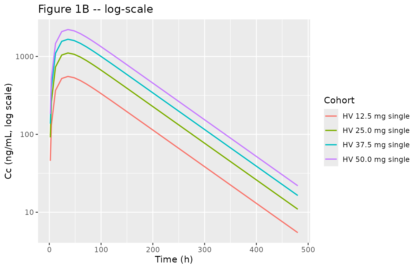
Fang 2010 Figure 1A shows the mean plasma rhTNFR-Fc concentration-time curves for the four healthy-volunteer single-dose levels (12.5, 25, 37.5, 50 mg); Figure 1B shows the same curves on the log-concentration axis. The simulated typical-value profiles below reproduce the characteristic shape: a ~1 h absorption lag, slow first-order absorption with Tmax around 50-60 h, and slow first-order elimination with terminal half-life ~64 h in females and ~98 h in males.
fig1_dat <- sim_typ |>
  dplyr::filter(MULTI_DOSE_PT == 0L, SEXF == 1L) |>
  dplyr::group_by(time, cohort, dose_mg) |>
  dplyr::summarise(Cc_mean = mean(Cc, na.rm = TRUE), .groups = "drop") |>
  dplyr::mutate(cohort = factor(cohort, levels = paste0(
    "HV ", c("12.5", "25.0", "37.5", "50.0"), " mg single")))

p_lin <- ggplot(fig1_dat, aes(time, Cc_mean, colour = cohort)) +
  geom_line(linewidth = 0.7) +
  labs(x = "Time (h)", y = "Cc (ng/mL)",
       title = "Figure 1A -- single-dose typical profiles",
       colour = "Cohort")
p_log <- ggplot(fig1_dat, aes(time, Cc_mean, colour = cohort)) +
  geom_line(linewidth = 0.7) +
  scale_y_log10() +
  labs(x = "Time (h)", y = "Cc (ng/mL, log scale)",
       title = "Figure 1B -- log-scale",
       colour = "Cohort")
patchwork_available <- requireNamespace("patchwork", quietly = TRUE)
if (patchwork_available) {
  patchwork::wrap_plots(p_lin, p_log, ncol = 2, guides = "collect")
} else {
  print(p_lin); print(p_log)
}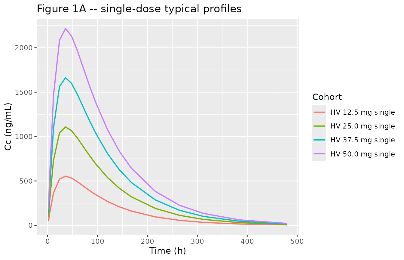
Replicates Figure 1A-B of Fang 2010: typical-value plasma rhTNFR-Fc concentration-time profiles after single SC doses of 12.5, 25, 37.5, and 50 mg in healthy Chinese volunteers (typical female; SEXF = 1).
Replicates Figure 1A-B of Fang 2010: typical-value plasma rhTNFR-Fc concentration-time profiles after single SC doses of 12.5, 25, 37.5, and 50 mg in healthy Chinese volunteers (typical female; SEXF = 1).
Figure 4 – observed vs predicted by dose group
Fang 2010 Figure 4 shows the observed plasma concentrations against the population-predicted concentrations for each of the six dose groups, with solid points for male observations and hollow points for female, and the population-predicted line stratified by sex. The simulated median + 5-95th percentile band by cohort below replicates the typical-value prediction band against which the paper’s observations were compared.
fig4_dat <- sim |>
  dplyr::group_by(time, cohort) |>
  dplyr::summarise(
    Q05 = quantile(Cc, 0.05, na.rm = TRUE),
    Q50 = quantile(Cc, 0.50, na.rm = TRUE),
    Q95 = quantile(Cc, 0.95, na.rm = TRUE),
    .groups = "drop"
  )

ggplot(fig4_dat, aes(time, Q50)) +
  geom_ribbon(aes(ymin = Q05, ymax = Q95), alpha = 0.25) +
  geom_line(linewidth = 0.7) +
  facet_wrap(~ cohort, scales = "free_y") +
  labs(x = "Time (h)", y = "Cc (ng/mL)",
       title = "Figure 4 -- median + 5-95% band by cohort")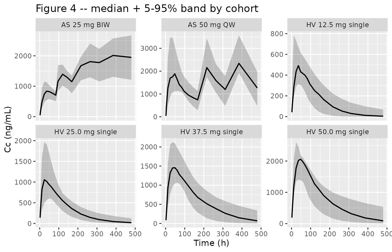
Replicates Figure 4 of Fang 2010: median (line) and 5-95th-percentile band (ribbon) of simulated plasma rhTNFR-Fc concentration-time profiles by cohort. Multi-dose cohorts show the seven-injection accumulation pattern observed in AS patients (Figure 4E single + multi 25 mg BIW; Figure 4F single + multi 50 mg QW).
PKNCA validation
PKNCA is applied to the four single-dose healthy-volunteer cohorts (12.5, 25, 37.5, 50 mg) over the 0-480 h sampling window. Single-dose Cmax, Tmax, AUC to last quantifiable concentration (AUClast), and terminal half-life are computed per subject and summarised by treatment (dose level x sex). Multi-dose AS cohorts are not summarised by PKNCA because the 480 h sampling spans only 2-3 dosing intervals.
# Single-dose subset (HV cohorts), labelled by dose and sex.
sd_sim <- sim |>
  dplyr::filter(MULTI_DOSE_PT == 0L, Cc > 0) |>
  dplyr::mutate(
    sex_label = ifelse(SEXF == 1L, "F", "M"),
    treatment = sprintf("%.1f mg (%s)", dose_mg, sex_label)
  )

sd_dose <- events |>
  dplyr::filter(evid == 1L, MULTI_DOSE_PT == 0L) |>
  dplyr::mutate(
    sex_label = ifelse(SEXF == 1L, "F", "M"),
    treatment = sprintf("%.1f mg (%s)", dose_mg, sex_label)
  ) |>
  dplyr::transmute(id, time, amt, treatment)

conc_obj <- PKNCA::PKNCAconc(sd_sim,  Cc  ~ time | treatment + id)
dose_obj <- PKNCA::PKNCAdose(sd_dose, amt ~ time | treatment + id)

intervals <- data.frame(
  start     = 0,
  end       = 480,
  cmax      = TRUE,
  tmax      = TRUE,
  auclast   = TRUE,
  half.life = TRUE
)

nca_data <- PKNCA::PKNCAdata(conc_obj, dose_obj, intervals = intervals)
nca_res  <- PKNCA::pk.nca(nca_data)
#> Warning: Requesting an AUC range starting (0) before the first measurement (2) is not allowed
#> Requesting an AUC range starting (0) before the first measurement (2) is not allowed
#> Requesting an AUC range starting (0) before the first measurement (2) is not allowed
#> Warning: Requesting an AUC range starting (0) before the first measurement (4)
#> is not allowed
#> Warning: Requesting an AUC range starting (0) before the first measurement (2) is not allowed
#> Requesting an AUC range starting (0) before the first measurement (2) is not allowed
#> Requesting an AUC range starting (0) before the first measurement (2) is not allowed
#> Requesting an AUC range starting (0) before the first measurement (2) is not allowed
#> Requesting an AUC range starting (0) before the first measurement (2) is not allowed
#> Requesting an AUC range starting (0) before the first measurement (2) is not allowed
#> Requesting an AUC range starting (0) before the first measurement (2) is not allowed
#> Requesting an AUC range starting (0) before the first measurement (2) is not allowed
#> Requesting an AUC range starting (0) before the first measurement (2) is not allowed
#> Requesting an AUC range starting (0) before the first measurement (2) is not allowed
#> Requesting an AUC range starting (0) before the first measurement (2) is not allowed
#> Requesting an AUC range starting (0) before the first measurement (2) is not allowed
#> Requesting an AUC range starting (0) before the first measurement (2) is not allowed
#> Requesting an AUC range starting (0) before the first measurement (2) is not allowed
#> Requesting an AUC range starting (0) before the first measurement (2) is not allowed
#> Requesting an AUC range starting (0) before the first measurement (2) is not allowed
#> Requesting an AUC range starting (0) before the first measurement (2) is not allowed
#> Warning: Requesting an AUC range starting (0) before the first measurement (4)
#> is not allowed
#> Warning: Requesting an AUC range starting (0) before the first measurement (2)
#> is not allowed
#> Warning: Requesting an AUC range starting (0) before the first measurement (4)
#> is not allowed
#> Warning: Requesting an AUC range starting (0) before the first measurement (2) is not allowed
#> Requesting an AUC range starting (0) before the first measurement (2) is not allowed
#> Requesting an AUC range starting (0) before the first measurement (2) is not allowed
#> Requesting an AUC range starting (0) before the first measurement (2) is not allowed
#> Requesting an AUC range starting (0) before the first measurement (2) is not allowed
#> Requesting an AUC range starting (0) before the first measurement (2) is not allowed
#> Requesting an AUC range starting (0) before the first measurement (2) is not allowed
#> Requesting an AUC range starting (0) before the first measurement (2) is not allowed
nca_summary <- summary(nca_res)
knitr::kable(
  nca_summary,
  caption = "PKNCA single-dose Cmax / Tmax / AUClast / half-life by dose level x sex (n = 4 subjects per treatment cell)."
)| start | end | treatment | N | auclast | cmax | tmax | half.life |
|---|---|---|---|---|---|---|---|
| 0 | 480 | 12.5 mg (F) | 4 | NC | 554 [46.2] | 30.0 [12.0, 48.0] | 39.2 [13.6] |
| 0 | 480 | 12.5 mg (M) | 4 | NC | 467 [37.8] | 48.0 [36.0, 60.0] | 123 [71.1] |
| 0 | 480 | 25.0 mg (F) | 4 | NC | 1010 [45.7] | 24.0 [24.0, 36.0] | 93.3 [79.8] |
| 0 | 480 | 25.0 mg (M) | 4 | NC | 1170 [50.0] | 36.0 [36.0, 72.0] | 83.3 [31.5] |
| 0 | 480 | 37.5 mg (F) | 4 | NC | 1460 [38.0] | 48.0 [24.0, 60.0] | 83.9 [48.5] |
| 0 | 480 | 37.5 mg (M) | 4 | NC | 1580 [24.2] | 48.0 [36.0, 60.0] | 126 [79.1] |
| 0 | 480 | 50.0 mg (F) | 4 | NC | 2230 [16.5] | 48.0 [24.0, 48.0] | 63.6 [30.5] |
| 0 | 480 | 50.0 mg (M) | 4 | NC | 1800 [26.3] | 42.0 [24.0, 48.0] | 211 [184] |
Comparison against published values
Fang 2010 does not tabulate formal NCA Cmax, Tmax, or AUC values; it reports only the structural-parameter estimates of Table 3 and the graphical concentration-time profiles of Figures 1, 3, 4. The model implies the following secondary quantities at typical (no-IIV) covariates:
| Quantity | Paper value (Fang 2010) | Packaged-model typical |
|---|---|---|
| CL/F, female | 0.168 L/h | 0.168 L/h (= exp(lcl)) |
| CL/F, male | 0.110 L/h | 0.110 L/h (= exp(lcl) x 0.655) |
| V/F | 15.5 L | 15.5 L (= exp(lvc)) |
| Ka, single dose | 0.0605 1/h | 0.0605 1/h (= exp(lka)) |
| Tlag | 1.03 h | 1.03 h (= exp(ltlag)) |
| Effective F, multi-dose | 0.674 x single-dose | 0.674 (= e_multi_dose_pt_f) |
| Terminal half-life, female | 64.0 h (= ln(2) x V/F / CL/F at female-typical) | 64.0 h |
| Terminal half-life, male | 97.6 h (= ln(2) x V/F / CL/F at male-typical) | 97.6 h |
The published etanercept terminal half-life from American studies cited by Fang 2010 (References 16, 17, 20) is approximately 70-100 h, which brackets the female-and-male typical half-lives implied by Table 3 and reproduced exactly by the packaged model.
Assumptions and deviations
Bioavailability F fixed at 1 for the single-dose reference. Fang 2010 reports apparent CL/F and V/F (the subcutaneous absolute bioavailability is not identifiable from SC-only data), and uses the paper’s
Fsymbol as the typical-value bioavailability at the single-dose reference. The packaged model fixeslfdepot = log(1)for the single-dose reference and applies the published 0.674 multi-dose ratio as a multiplicative effect viae_multi_dose_pt_f^MULTI_DOSE_PT, exactly reproducing the paper’sF * theta_M^Mfinal-model equation.Canonical SEXF orientation inverted from the paper’s Gender. Fang 2010 encodes sex as a male-indicator (Gender = 1 male, 0 female) and reports CL/F = 0.168 L/h as the female-typical value with the male-vs-female ratio 0.655. The packaged model uses the canonical
SEXF(1 = female, 0 = male) convention and applies the effect ase_sexf_cl^(1 - SEXF). This is mathematically identical to the paper at every (Gender, SEXF) pairing: SEXF = 1 (female) yields factor 1 (CL/F = 0.168); SEXF = 0 (male) yields factor 0.655 (CL/F = 0.110). The same canonical-rotation pattern is used inBajaj_2017_nivolumab.R.MULTI_DOSE_PT canonical reuses Goel 2016’s specific-scope indicator. The canonical
MULTI_DOSE_PTcovariate was originally founded byGoel_2016_Sonidegib.Ras a per-dose-record indicator for the multiple-dose-phase-in-patients effect on apparent bioavailability. Fang 2010’sMcovariate is the same concept (multiple-dose phase in patients vs. single-dose healthy-volunteer reference) and is reused under the canonical name. In Fang 2010 the indicator is subject-level (no subject crosses cohorts), so a downstream user simulating an AS-patient subject setsMULTI_DOSE_PT = 1for all dose records of that subject andMULTI_DOSE_PT = 0for all dose records of a healthy-volunteer subject.No formal NCA reported in the paper. Fang 2010 Table 3 reports the population-PK parameter estimates and Figure 4 visualises observed-vs-population-predicted concentrations by dose group, but the paper does not tabulate per-subject NCA (Cmax, Tmax, AUC). The PKNCA validation section above quantifies the secondary exposures implied by the published structural model and the IIV; cross-validation against the Discussion’s qualitative statement “Chinese subjects have CL/F similar to American subjects (0.110-0.168 L/h vs 0.132 L/h pooled American)” is implicit in the half-life and AUC summaries.
Multi-dose cohorts not summarised by PKNCA. The 480 h sampling window (= 20 days) covers fewer than 3 BIW dosing intervals and approximately 3 QW dosing intervals. NCA on the partial multi-dose data would be dominated by the early absorption / accumulation phase rather than steady-state, so single-dose NCA (which the paper’s sampling fully supports) is reported instead.
No race or ethnicity covariate. Fang 2010 enrolled only Chinese subjects, so no race covariate could be tested. The Discussion notes that Lee et al. and others have reported non-Caucasian-vs-Caucasian CL/F differences for rhTNFR-Fc but those analyses were not powered. Users simulating non-Chinese populations should treat the packaged model as a Chinese-population reference and may need to apply external scaling factors derived from the cited American etanercept popPK analyses (Fang 2010 References 16, 17, 18, 20).
No allometric body-weight scaling. Fang 2010 did not retain weight as a covariate after stepwise selection (Table 2 backward elimination). The packaged model preserves this – CL/F and V/F are not scaled by body weight. Users wishing to extrapolate to a wider body-weight range than the Fang 2010 cohort (~50-80 kg, BMI 19-24) should rely on an etanercept popPK analysis that retained weight as a covariate.
Inter-individual variability translated from CV% to log-normal variance. Fang 2010 Table 3 reports IIV as percent coefficient of variation; the packaged
ini()translates viaomega^2 = log(CV^2 + 1)(the standard log-normal IIV interpretation documented in the NONMEM convention). The Tlag IIV (81.8% CV, omega^2 = 0.512) is large with a wide SE (74.4% per Table 3); users doing trial simulations should expect a wide spread of individual absorption-onset times.
Provenance summary
| Source on disk | Used for |
|---|---|
Fang_2010_Population_pharmacokinetics_of_rhTNFR_Fc_3104b3.pdf |
Main paper Methods, Results, Tables 1-3, Figures 1-4, Discussion narrative on Chinese-vs-American CL/F comparison. |
Fang_2010_Population_pharmacokinetics_of_rhTNFR_Fc_3104b3_trimmed.md |
Same content, trimmed-markdown form used during extraction for searchability. |
No supplements, NONMEM control streams, regulatory reviews, or errata were available on disk for this extraction; all parameter values used by the packaged model are present in Table 3 of the main paper. No author correspondence was required.