Methotrexate (Wang 2019)
Source:vignettes/articles/Wang_2019_methotrexate.Rmd
Wang_2019_methotrexate.RmdModel and source
- Citation: Wang Z, Zhang N, Chen C, Chen S, Xu J, Zhou Y, Zhao X, Cui Y (2019). Influence of the OATP Polymorphism on the Population Pharmacokinetics of Methotrexate in Chinese Patients. Curr Drug Metab 20(7):592-600. doi:10.2174/1389200220666190701094756.
- Description: One-compartment population PK model with first-order absorption and linear elimination for low-dose oral methotrexate in Chinese adults with rheumatoid arthritis (Wang 2019; n = 71 patients, 85 mostly trough concentrations). Clearance depends on the SLCO1B1 (OATP1B1) c.388A>G (rs2306283) genotype through multiplicative factors for the 388A/G heterozygote and 388G/G homozygote relative to 388A/A. Volume, absorption rate and bioavailability are fixed. Exponential between-subject variability on clearance only, and combined proportional plus additive residual error.
- Article: Curr Drug Metab 2019;20(7):592-600 (open access via PMC6857112)
Wang 2019 is a small NONMEM analysis of low-dose oral methotrexate in Chinese adults with rheumatoid arthritis, aimed at the effect of hepatic uptake transporter (OATP1B1 / OATP1B3) polymorphisms on apparent clearance. The final model is one-compartment with first-order absorption; only the SLCO1B1 c.388A>G (rs2306283) genotype survived backward deletion as a covariate on clearance.
Read the “Assumptions, deviations and errata” section before using this model. The final-model equation as printed in the paper is not the model the table parameters describe, and the dose regimen of the cohort is not reported.
Population
71 patients with rheumatoid arthritis treated with low-dose methotrexate at Peking University First Hospital contributed 85 concentrations, most of them trough samples (Section 3.1 and Discussion). Table 1 reports body weight 59.4 (SD 10.7) kg, age 48.0 (SD 15.2) years, height 1.61 (SD 0.06) m and BSA 1.6 (SD 0.16) m^2, and prints sex as ‘GEND(Male/Female) 60/11’. SLCO1B1 rs2306283 genotypes were GG 43, AG 22 and AA 6 (Table 2; Table 1 prints 42/23/6). Concentrations were measured by LC-MS with an LLOQ of 0.5 ng/mL (Section 2.2).
Source trace
| Element | Value | Source |
|---|---|---|
| Structure | 1-compartment, first-order absorption and elimination | Abstract; Section 2.4; Discussion |
lcl (388A/A) |
7.75 L/h | Table 3, theta1 |
lvc |
32.8 L (FIX) | Table 3, theta2; final-model equation |
lka |
1.69 1/h (FIX) | Table 3, theta3 (unit printed ‘h/L’); final-model equation |
lfdepot |
0.704 (FIX) | Table 3, theta4; final-model equation |
e_snp_slco1b1_rs2306283_hom_cl (388G/G) |
0.805 | Table 3, theta5; equation ‘RS230 = 1’ |
e_snp_slco1b1_rs2306283_het_cl (388A/G) |
0.647 | Table 3, theta6; equation ‘RS230 = 2’ |
etalcl |
0.167 (FIX, variance) | Table 3, omega CL |
propSd |
sqrt(0.713) | Table 3, sigma1 (pro) |
addSd |
sqrt(2.83) ng/mL | Table 3, sigma2 (add) |
| Genotype coding | RS230: 1 = G/G, 2 = A/G, 3 = A/A | Abstract; Section 3.3 equation |
| IIV form | P = PTV x exp(eta) | Equation 1 |
Typical clearance by genotype
mod <- readModelDb("Wang_2019_methotrexate")
ui <- rxode2::rxode(mod)
#> ℹ parameter labels from comments will be replaced by 'label()'
th <- ui$theta

geno <- tibble::tibble(
  genotype = c("388A/A", "388A/G", "388G/G"),
  SNP_SLCO1B1_RS2306283_HET = c(0, 1, 0),
  SNP_SLCO1B1_RS2306283_HOM = c(0, 0, 1),
  n_cohort = c(6, 22, 43)
) |>
  mutate(
    cl = exp(th[["lcl"]]) *
      th[["e_snp_slco1b1_rs2306283_het_cl"]]^SNP_SLCO1B1_RS2306283_HET *
      th[["e_snp_slco1b1_rs2306283_hom_cl"]]^SNP_SLCO1B1_RS2306283_HOM,
    pct_vs_AA = 100 * (cl / cl[1] - 1)
  )
knitr::kable(geno |> dplyr::select(genotype, n_cohort, cl, pct_vs_AA), digits = 2)| genotype | n_cohort | cl | pct_vs_AA |
|---|---|---|---|
| 388A/A | 6 | 7.75 | 0.0 |
| 388A/G | 22 | 5.01 | -35.3 |
| 388G/G | 43 | 6.24 | -19.5 |
Two independent statements in the paper check this parameterisation:
- The base model (no covariates) estimated a population CL/F of 5.98 L/h (Section 3.2). Weighting the final-model genotype clearances by the Table 2 genotype counts gives the cohort-average clearance, which should land close to that value.
- The Discussion states that CL/F ‘diminished by 32.3% in patients carrying the OATP1B1-388AG and 17.8% in patients carrying the OATP1B1-388GG genotypes’ compared with 388AA.
cl_mix <- with(geno, sum(cl * n_cohort) / sum(n_cohort))
cl_mix
#> [1] 5.987039
stopifnot(
  abs(cl_mix / 5.98 - 1) < 0.03,
  # Direction and ordering of the Discussion's quoted reductions:
  geno$pct_vs_AA[2] < geno$pct_vs_AA[3],
  geno$pct_vs_AA[3] < 0,
  abs(geno$pct_vs_AA[2] - (-32.3)) < 4,
  abs(geno$pct_vs_AA[3] - (-17.8)) < 4
)
The genotype-weighted clearance is 5.99 L/h against the base model’s 5.98 L/h, and the modelled reductions (-35.3% for A/G, -19.5% for G/G) reproduce the Discussion’s -32.3% / -17.8% to within about 3 percentage points. The literal printed equation (see Errata) predicts reductions of only -5.7% and -3.2% and a cohort-average clearance near 8.8 L/h, and fails both checks.
Simulation
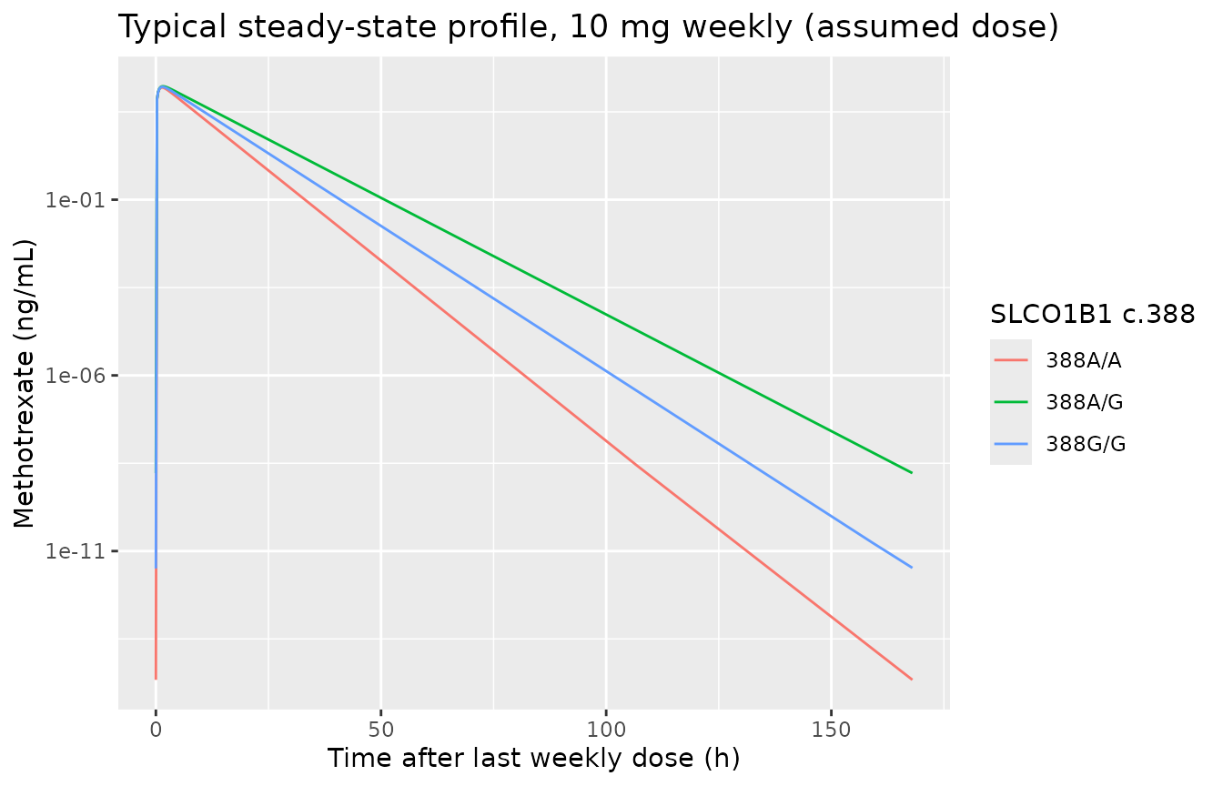
The paper does not report the dose. The simulations below assume 10 mg oral once weekly, a typical low-dose RA regimen, to steady state (6 weeks); this is an illustration of the model, not a reproduction of the study design.
dose_mg <- 10
tau <- 168
n_dose <- 6
t_last <- (n_dose - 1) * tau

ev_typ <- geno |>
  mutate(id = seq_len(n())) |>
  select(id, genotype, starts_with("SNP_")) |>
  tidyr::crossing(
    bind_rows(
      tibble::tibble(time = (0:(n_dose - 1)) * tau, amt = dose_mg, evid = 1, cmt = "depot"),
      tibble::tibble(time = t_last + c(0, seq(0.25, tau, by = 0.25)), amt = 0, evid = 0, cmt = "central")
    )
  ) |>
  arrange(id, time, desc(evid)) |>
  as.data.frame()

sim_typ <- rxode2::rxSolve(rxode2::zeroRe(mod), ev_typ, keep = "genotype") |>
  as.data.frame()
#> ℹ parameter labels from comments will be replaced by 'label()'
#> ℹ omega/sigma items treated as zero: 'etalcl'
#> Warning: multi-subject simulation without without 'omega'

ggplot(filter(sim_typ, time >= t_last), aes(time - t_last, Cc, colour = genotype)) +
  geom_line() +
  scale_y_log10() +
  labs(
    x = "Time after last weekly dose (h)", y = "Methotrexate (ng/mL)",
    colour = "SLCO1B1 c.388",
    title = "Typical steady-state profile, 10 mg weekly (assumed dose)"
  )
Stochastic cohort
set.seed(2019)
rxode2::rxSetSeed(2019)
n_sub <- 150
cohort <- tibble::tibble(
  id = seq_len(n_sub),
  genotype = sample(c("388A/A", "388A/G", "388G/G"), n_sub, replace = TRUE, prob = c(6, 22, 43))
) |>
  mutate(
    SNP_SLCO1B1_RS2306283_HET = as.numeric(genotype == "388A/G"),
    SNP_SLCO1B1_RS2306283_HOM = as.numeric(genotype == "388G/G")
  )
ev_vpc <- cohort |>
  tidyr::crossing(
    bind_rows(
      tibble::tibble(time = (0:(n_dose - 1)) * tau, amt = dose_mg, evid = 1, cmt = "depot"),
      tibble::tibble(time = t_last + c(0, 0.5, 1, 1.5, 2, 3, 4, 6, 8, 12, 16, 24), amt = 0, evid = 0, cmt = "central")
    )
  ) |>
  arrange(id, time, desc(evid)) |>
  as.data.frame()
sim_vpc <- rxode2::rxSolve(mod, ev_vpc, keep = "genotype") |> as.data.frame()
#> ℹ parameter labels from comments will be replaced by 'label()'

sim_vpc |>
  filter(time >= t_last) |>
  group_by(tad = time - t_last) |>
  summarise(
    p05 = quantile(Cc, 0.05), p50 = median(Cc), p95 = quantile(Cc, 0.95),
    .groups = "drop"
  ) |>
  ggplot(aes(tad, p50)) +
  geom_ribbon(aes(ymin = pmax(p05, 0.1), ymax = p95), alpha = 0.3) +
  geom_line() +
  scale_y_log10() +
  labs(
    x = "Time after last weekly dose (h)", y = "Methotrexate (ng/mL)",
    title = "Individual predictions (IPRED): median and 90% interval, 10 mg weekly (assumed dose)"
  )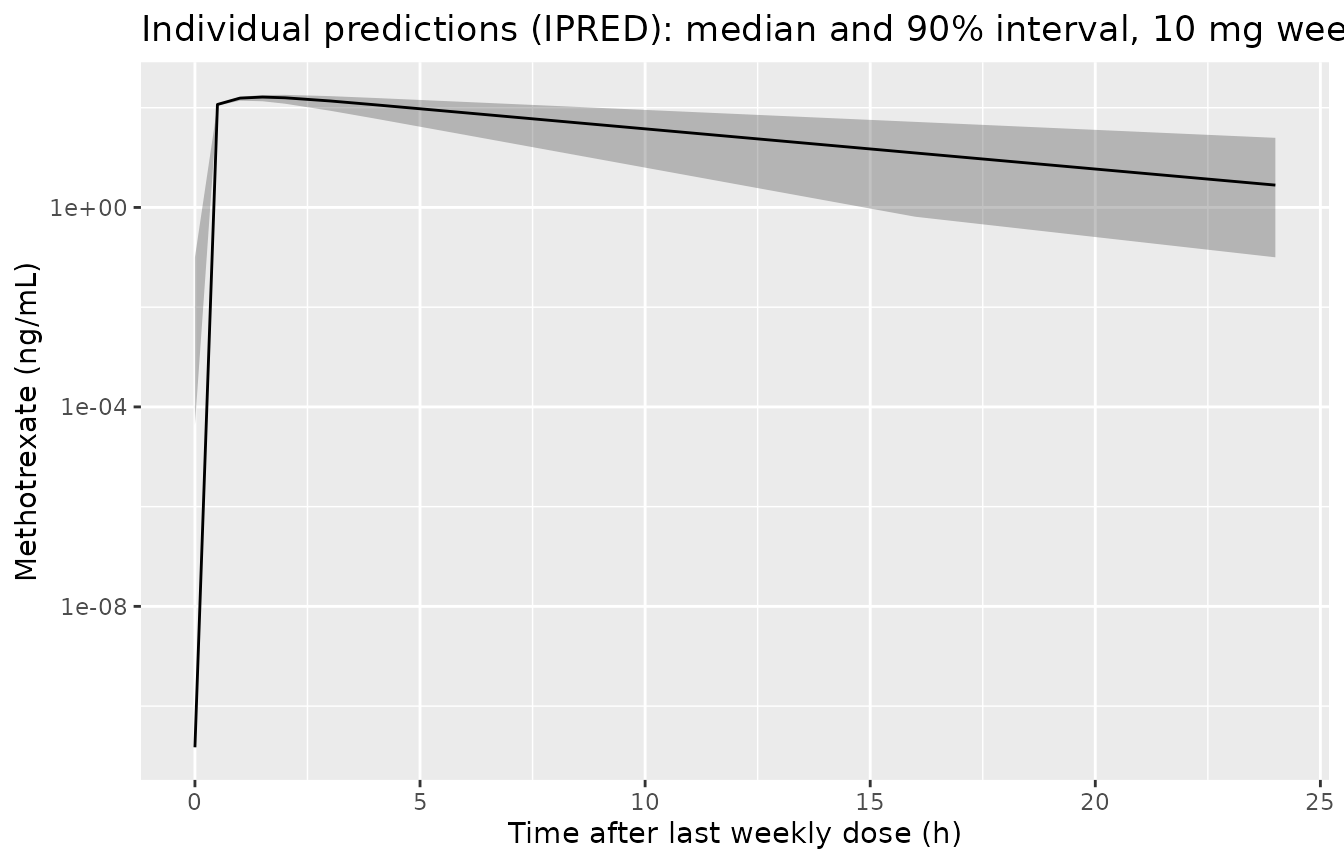
The paper publishes goodness-of-fit plots only (Figs 1-4), with observed concentrations mostly below 20 ng/mL and population predictions up to about 250 ng/mL (Fig 3). A 10 mg dose predicts a typical peak of roughly 155-170 ng/mL across genotypes, compatible with that range; no VPC was published to compare against.
PKNCA validation
The paper reports no NCA. The check is instead against the model’s
own closed form: at steady state the dosing-interval AUC equals
F x Dose / CL, exactly, for every genotype.
conc_df <- sim_typ |>
  filter(time >= t_last, !is.na(Cc)) |>
  mutate(tad = time - t_last) |>
  select(id, genotype, time = tad, Cc)
dose_df <- tibble::tibble(id = geno |> mutate(id = seq_len(n())) |> pull(id), genotype = geno$genotype, time = 0, amt = dose_mg)

conc_obj <- PKNCA::PKNCAconc(conc_df, Cc ~ time | genotype + id)
dose_obj <- PKNCA::PKNCAdose(dose_df, amt ~ time | genotype + id)
intervals <- data.frame(start = 0, end = tau, auclast = TRUE, cmax = TRUE, tmax = TRUE, half.life = TRUE)
nca <- PKNCA::pk.nca(PKNCA::PKNCAdata(conc_obj, dose_obj, intervals = intervals))

nca_wide <- as.data.frame(nca$result) |>
  select(genotype, PPTESTCD, PPORRES) |>
  tidyr::pivot_wider(names_from = PPTESTCD, values_from = PPORRES) |>
  left_join(geno |> select(genotype, cl), by = "genotype") |>
  mutate(
    auc_closed = 1000 * exp(th[["lfdepot"]]) * dose_mg / cl, # ng h/mL
    pct_diff = 100 * (auclast / auc_closed - 1)
  )
nca_wide |>
  select(genotype, cmax, tmax, half.life, auclast, auc_closed, pct_diff) |>
  dplyr::rename(
    "SLCO1B1 c.388" = genotype, "Cmax (ng/mL)" = cmax, "Tmax (h)" = tmax,
    "t1/2 (h)" = half.life, "AUCtau PKNCA (ng h/mL)" = auclast,
    "AUCtau = F x Dose / CL (ng h/mL)" = auc_closed, "% diff" = pct_diff
  ) |>
knitr::kable(digits = 2)| SLCO1B1 c.388 | Cmax (ng/mL) | Tmax (h) | t1/2 (h) | AUCtau PKNCA (ng h/mL) | AUCtau = F x Dose / CL (ng h/mL) | % diff |
|---|---|---|---|---|---|---|
| 388A/A | 155.53 | 1.25 | 2.96 | 906.33 | 908.39 | -0.23 |
| 388A/G | 168.92 | 1.50 | 4.53 | 1401.99 | 1404.00 | -0.14 |
| 388G/G | 162.65 | 1.50 | 3.65 | 1126.40 | 1128.43 | -0.18 |
PKNCA reproduces the closed-form AUC to under 1% for every genotype
(a deterministic typical-value solve, so a tight bound is appropriate),
and the terminal half-life equals log(2) x V / CL (2.93 /
4.53 / 3.64 h).
Assumptions, deviations and errata
-
Final-model clearance equation. Section 3.3 prints
RS230 = 1 : CL = 7.75 x e^(0.167 x 0.805),RS230 = 2 : ... e^(0.167 x 0.647)andRS230 = 3 : ... e^(0.167 x 1), where 0.167 is the omega of CL and 0.805 / 0.647 are theta5 / theta6. Read literally this puts the IIV variance inside the typical value and makes the genotype effect tiny (-3% / -6%). It is encoded instead asCL = theta1 x theta_genotype x exp(eta_CL), the usual NONMEM multiplicative categorical form, because (a) the genotype-weighted clearance then matches the base-model CL/F of 5.98 L/h, and (b) the resulting -35% / -19% reductions match the Discussion’s quoted -32.3% / -17.8% far better than the literal reading’s -6% / -3%. The residual gap of about 3 points to the Discussion’s numbers is not explained by the paper (the bootstrap medians 0.589 / 0.760 give larger, not smaller, reductions). -
Abstract equation is a different model. The
Abstract prints
CL (L/h) = 8.25 x e^(0.167 x SNP)with SNP = 1, 2, 3 for G/G, A/G, A/A. It matches neither Table 3 nor the Section 3.3 equation, and is not used. -
F = 0.704 applied. Table 3 and the final-model
equation both list F = 0.704 FIX alongside parameters labelled CL/F and
V/F. F is applied to the depot here, as printed, so
clandvccarry the Table 3 values; the apparent oral clearance of this implementation is thereforecl / 0.704. The source of the fixed V, Ka and F values is not cited in the paper. - Ka unit. Table 3 prints ‘Ka (h/L)’; the abstract and the model structure make it 1/h.
-
Residual and IIV scale. Table 3 gives bare numbers.
The sigma rows are treated as NONMEM
$SIGMAvariances: their bootstrap 95% CI relative widths (0.69 for proportional, 0.93 for additive, on 85 observations) match the variance prediction (about 0.60) and not the SD prediction (about 0.30). An additive SD of 2.83 ng/mL would also be large next to observations mostly below 5 ng/mL (Figs 1-2). omega CL = 0.167 is taken as a variance by the same NONMEM convention (CV about 43%); it is FIXED in the paper and no source is given. Section 2.4 says the residual model is proportional; Table 3 estimates both a proportional and an additive term, and both are encoded. -
Additive-error units. Assumed ng/mL, the assay’s
reporting unit (Section 2.2); the model outputs
Ccin ng/mL from mg doses and L volumes. - IIV on V, Ka, F are ‘0 FIX’ in Table 3 and are omitted.
- Dose regimen. Not reported. The 10 mg weekly regimen in the simulations is an assumption for illustration only.
-
Sex split. Table 1 prints ‘GEND(Male/Female)
60/11’;
populationfollows the print, but a predominantly male RA cohort is unusual and the columns may be transposed. - Genotype counts. Table 1 (42/23/6) and Table 2 (43/22/6) differ by one subject between G/G and A/G; Table 2 is used for the cohort weighting.