Praziquantel in pregnancy and lactation (Bustinduy 2020)

Model and source

#> ℹ parameter labels from comments will be replaced by 'label()'

• Citation: Bustinduy AL, Kolamunnage-Dona R, Mirochnick MH, Capparelli EV, Tallo V, Acosta LP, Olveda RM, Friedman JF, Hope WW. Population pharmacokinetics of praziquantel in pregnant and lactating Filipino women infected with Schistosoma japonicum. Antimicrob Agents Chemother. 2020;64(9):e00566-20. doi:10.1128/AAC.00566-20. PMCID: PMC7449211.

• Description: Two-compartment oral population PK model with a first-order absorption (gut) compartment, an absorption lag and a reversible breast-milk compartment for praziquantel (racemic, total PZQ) in 45 Filipino women with Schistosoma japonicum infection – 15 in early pregnancy (12-16 weeks gestation), 15 in late pregnancy (30-36 weeks) and 15 lactating postpartum women (5-7 months postpartum) – given 60 mg/kg as two 30 mg/kg oral doses 3 h apart. Plasma and breast milk were co-modelled non-parametrically with NPAG in Pmetrics. Drug moves from central to milk and back with first-order rate constants and is NOT eliminated through milk (the authors’ identifiability choice), so the milk compartment behaves as a sampled second peripheral compartment with its own apparent volume. Clearance and volumes are apparent (CL/F, Vc/F, Vmilk/F); bioavailability was not estimated. No covariate was retained: weight showed no relationship with CL/F or Vc/F, and the higher CL/F of early-pregnancy women was reported only as a post hoc comparison of Bayesian posteriors, not built into the model. Residual variability is fixed(0) because the Pmetrics assay-error model was not published.

• Article: https://doi.org/10.1128/AAC.00566-20 (open access; PMCID PMC7449211)

This is the first description of praziquantel (PZQ) pharmacokinetics in pregnant and lactating women. It was nested in a randomised controlled trial of PZQ in pregnancy in Leyte, Philippines. Women with Schistosoma japonicum received the trial regimen of 60 mg/kg, given as two 30 mg/kg oral doses 3 h apart. Plasma PK was studied in three cohorts of 15 women each: early pregnancy, late pregnancy and lactating postpartum. Breast milk was also sampled in the lactating cohort. Plasma and milk were co-modelled with the non-parametric NPAG algorithm in Pmetrics.

The same senior author’s group published the paediatric model Bustinduy_2016_praziquantel (Ugandan children, S. mansoni). The two models share the gut / central / peripheral skeleton and Pmetrics parameter names. This paper adds a breast-milk compartment.

Population

45 women entered the PK analysis. Forty-seven were enrolled; two early-pregnancy women vomited shortly after dosing and were not sampled. The Table 1 baseline data cover all 47 enrolled women. Median age was 24.0 years (range 18-44) and mean weight 48.5 kg (SD 7.69); cohort means were 47.6, 51.5 and 46.6 kg. All participants were Asian (Filipino) and non-Hispanic. Infection intensity was low (< 100 eggs per gram) in 46 of the 47 and moderate in one. The early-pregnancy cohort was 12-16 weeks gestation, the late-pregnancy cohort 30-36 weeks, and the lactating cohort 5-7 months postpartum.

Population metadata carried in the model file.

Field	Value
species	human
n_subjects	45
n_studies	1
age_range	18-44 years
age_median	24.0 years (mean 25.5, SD 6.39; 47 enrolled)
weight_range	approximately 36-63 kg (read from Fig. 5; not tabulated)
weight_median	47.9 kg (median used for the Monte Carlo simulations); mean 48.5 kg (SD 7.69; 47 enrolled)
sex_female_pct	100
race_ethnicity	Asian (Filipino), 100%
disease_state	Stool-positive Schistosoma japonicum infection, otherwise healthy; infection intensity low (< 100 eggs per gram) in 46 of 47 enrolled and moderate in 1.
dose_range	60 mg/kg praziquantel given orally as two 30 mg/kg doses approximately 3 h apart, after a carbohydrate-rich snack. Absolute total doses about 2100-3800 mg (Fig. 6A).
regions	Philippines (northeastern Leyte)
reproductive_status	Early pregnancy 12-16 weeks gestation (n = 15 analysed; 17 enrolled, 2 vomited and were not sampled), late pregnancy 30-36 weeks gestation (n = 15), lactating 5-7 months postpartum (n = 15).
notes	Baseline demographics from Table 1 (47 enrolled). Plasma sampled pre-dose and at 1, 2, 3 (before the second dose), 4, 5, 6, 7, 8, 9, 12, 15 and 24 h after the first dose; breast milk hand-expressed at 3, 6, 9, 12, 15 and 24 h in the lactating group only. LC-MS assay; LLOQ 31.3 ng/mL in plasma and 4.3 ng/mL in milk (Methods). Posterior CL/F was higher in early pregnancy (median about 425 L/h vs about 245 L/h; Fig. 6C) and AUC0-24 lower (median about 7 vs 11-12 mg*h/L; Fig. 6D), but this was not encoded as a covariate effect.

Source trace

All structural values are the mean of the NPAG parameter distribution in Table 2. The next section explains why the mean is used rather than the median.

Equation / parameter	Value	Source location
lka (Ka)	2.012 1/h	Table 2, row Ka (h-1), mean (median 0.395)
lcl (SCL/F)	324.075 L/h	Table 2, row SCL/F (liter/h), mean (median 277.447)
lvc (Vc/F)	183.006 L	Table 2, row Vc/F (liter), mean (median 142.618)
lk12 (Kcp)	19.313 1/h	Table 2, row Kcp (h-1), mean (median 18.941)
lk21 (Kpc)	15.816 1/h	Table 2, row Kpc (h-1), mean (median 13.996)
lk_central_milk (Kcb)	18.750 1/h	Table 2, row Kcb (h-1), mean (median 19.301)
lk_milk_central (Kbc)	17.816 1/h	Table 2, row Kbc (h-1), mean (median 17.077)
lvmilk (Vb/F)	612.130 L	Table 2, row Vb/F (liter), mean (median 563.802)
ltlag (Lag)	0.772 h	Table 2, row Lag (h), mean (median 0.868)
lfdepot (F)	fixed(log(1))	Not estimated; all clearances and volumes in Table 2 are /F
eta* variances	log(CV^2 + 1)	Table 2 CV (%) column (see identity check below)
propSd, addSd, propSd_Cmilk, addSd_Cmilk	fixed(0)	Not reported; see Errata
d/dt(depot), d/dt(central), d/dt(peripheral1), d/dt(milk)	n/a	Methods, equations (1)-(4), with the typesetting corrections listed in Errata
alag(depot)	n/a	Methods: “A lag function … was applied between the oral administration of PZQ and the appearance of drug in the central compartment”
Cc <- central / vc	n/a	Methods, output equation Y(1) (printed with X(1); see Errata)
Cmilk <- milk / vmilk	n/a	Methods, output equation Y(2) = X(4) / Vb
No covariates	n/a	Results: “Hence, covariates were not incorporated into the structural model”

Table 2 prints CV (%) alongside Mean and SD. For every row, SD / Mean reproduces the printed CV to the rounding of the printed SD. So the CV is on the linear scale, which supports the log(CV^2 + 1) conversion.

tab2 <- tibble::tribble(
  ~parameter, ~mean, ~median, ~sd, ~cv_pct,
  "Ka", 2.012, 0.395, 4.301, 213.750,
  "SCL/F", 324.075, 277.447, 175.373, 54.115,
  "Vc/F", 183.006, 142.618, 93.211, 50.933,
  "Kcp", 19.313, 18.941, 10.167, 52.644,
  "Kpc", 15.816, 13.996, 9.447, 59.733,
  "Kcb", 18.750, 19.301, 9.387, 50.067,
  "Kbc", 17.816, 17.077, 7.845, 44.031,
  "Vb/F", 612.130, 563.802, 395.661, 64.637,
  "Lag", 0.772, 0.868, 0.233, 30.202
) |>
  mutate(
    cv_from_sd_over_mean = 100 * sd / mean,
    omega2 = log((cv_pct / 100)^2 + 1)
  )

# The printed CV% is SD/mean on the linear scale. The largest gap is Lag (the SD
# is printed to only three digits, 0.233).
stopifnot(max(abs(tab2$cv_from_sd_over_mean - tab2$cv_pct)) < 0.05)

# The encoded omegas are exactly these values.
om <- diag(ui$omega)
stopifnot(max(abs(om - tab2$omega2)) < 1e-5)

tab2 |>
  dplyr::rename(
    "Parameter" = parameter,
    "Mean" = mean,
    "Median" = median,
    "SD" = sd,
    "CV% (printed)" = cv_pct,
    "100 x SD/mean" = cv_from_sd_over_mean,
    "omega^2 encoded" = omega2
  ) |>
  knitr::kable(digits = 4, caption = "Table 2 of Bustinduy 2020, with the CV% identity check.")

Table 2 of Bustinduy 2020, with the CV% identity check.

Parameter	Mean	Median	SD	CV% (printed)	100 x SD/mean	omega^2 encoded
Ka	2.012	0.395	4.301	213.750	213.7674	1.7172
SCL/F	324.075	277.447	175.373	54.115	54.1149	0.2568
Vc/F	183.006	142.618	93.211	50.933	50.9333	0.2306
Kcp	19.313	18.941	10.167	52.644	52.6433	0.2446
Kpc	15.816	13.996	9.447	59.733	59.7307	0.3051
Kcb	18.750	19.301	9.387	50.067	50.0640	0.2237
Kbc	17.816	17.077	7.845	44.031	44.0335	0.1772
Vb/F	612.130	563.802	395.661	64.637	64.6368	0.3491
Lag	0.772	0.868	0.233	30.202	30.1813	0.0873

Structural verification

These checks use typical values with the random effects zeroed. They do not depend on the simulated cohort, so they are tightly gated.

mod <- readModelDb("Bustinduy_2020_praziquantel")
mod_typ <- rxode2::zeroRe(mod)
#> ℹ parameter labels from comments will be replaced by 'label()'

p_mean <- c(
  ka = 2.012, cl = 324.075, vc = 183.006, kcp = 19.313, kpc = 15.816,
  kcb = 18.750, kbc = 17.816, vb = 612.130, tlag = 0.772
)
p_median <- c(
  ka = 0.395, cl = 277.447, vc = 142.618, kcp = 18.941, kpc = 13.996,
  kcb = 19.301, kbc = 17.077, vb = 563.802, tlag = 0.868
)
as_theta <- function(p) {
  c(
    lka = log(p[["ka"]]), lcl = log(p[["cl"]]), lvc = log(p[["vc"]]),
    lk12 = log(p[["kcp"]]), lk21 = log(p[["kpc"]]),
    lk_central_milk = log(p[["kcb"]]), lk_milk_central = log(p[["kbc"]]),
    lvmilk = log(p[["vb"]]), ltlag = log(p[["tlag"]])
  )
}

# The trial regimen: two 30 mg/kg oral doses 3 h apart. The paper's worked
# numbers use the median weight of 47.9 kg.
wt_ref <- 47.9
# The model declares two error endpoints (Cc and Cmilk), so every observation
# row must nominate one through `dvid`; both concentrations are returned as
# columns on every row regardless.
split_dose <- function(wt, tmax = 72, dt = 0.01) {
  rxode2::et(amt = 30 * wt, time = c(0, 3), cmt = "depot") |>
    rxode2::et(seq(0, tmax, by = dt), cmt = "central") |>
    as.data.frame() |>
    dplyr::mutate(dvid = ifelse(evid == 0, 1L, NA_integer_))
}
solve_typ <- function(theta, wt = wt_ref, tmax = 72) {
  rxode2::rxSolve(mod_typ, split_dose(wt, tmax),
    params = theta,
    returnType = "data.frame", rtol = 1e-10, atol = 1e-14
  )
}

typ <- solve_typ(as_theta(p_mean))
#> ℹ omega/sigma items treated as zero: 'etalka', 'etalcl', 'etalvc', 'etalk12', 'etalk21', 'etalk_central_milk', 'etalk_milk_central', 'etalvmilk', 'etaltlag'
dose_tot <- 60 * wt_ref

trap <- function(y, t) sum(diff(t) * (head(y, -1) + tail(y, -1)) / 2)

# 1. Mass balance. Milk has no elimination, so all drug leaves through CL and
#    AUC(0-inf) of plasma equals Dose / CL (F = 1). By 72 h the typical profile
#    is many half-lives down.
auc_p <- trap(typ$Cc, typ$time)
mb_err <- abs(auc_p / (dose_tot / p_mean[["cl"]]) - 1)
stopifnot(mb_err < 1e-3)

# 2. Milk partition identity. With no milk elimination, the milk AMOUNT
#    integrates to (Kcb / Kbc) x the central AMOUNT, so the concentration AUC
#    ratio is (Kcb / Kbc) x (Vc / Vb). This checks the sign fix to the printed
#    eq. (4). The printed sign would drive milk negative.
auc_m <- trap(typ$Cmilk, typ$time)
ratio_closed <- (p_mean[["kcb"]] / p_mean[["kbc"]]) * (p_mean[["vc"]] / p_mean[["vb"]])
ratio_err <- abs(auc_m / auc_p / ratio_closed - 1)
stopifnot(ratio_err < 1e-3, all(typ$Cmilk >= 0))

# 3. Absorption lag: nothing in plasma before Tlag.
stopifnot(all(typ$Cc[typ$time < p_mean[["tlag"]] - 1e-9] == 0))

# 4. The milk compartment is load-bearing for plasma: removing the milk
#    exchange changes the plasma profile.
no_milk <- solve_typ(replace(as_theta(p_mean), "lk_central_milk", log(1e-9)))
#> ℹ omega/sigma items treated as zero: 'etalka', 'etalcl', 'etalvc', 'etalk12', 'etalk21', 'etalk_central_milk', 'etalk_milk_central', 'etalvmilk', 'etaltlag'
milk_effect <- max(abs(no_milk$Cc - typ$Cc)) / max(typ$Cc)
stopifnot(milk_effect > 0.05)

tibble::tibble(
  Check = c(
    "Plasma AUC(0-72) recovers Dose / CL (rel. error)",
    "Milk:plasma AUC ratio vs (Kcb/Kbc)(Vc/Vb) (rel. error)",
    "Closed-form milk:plasma AUC ratio",
    "Plasma profile change when milk exchange is removed (fraction of Cmax)"
  ),
  Value = signif(c(mb_err, ratio_err, ratio_closed, milk_effect), 4)
) |>
  knitr::kable(caption = "Deterministic structural checks (all gated).")

Deterministic structural checks (all gated).

Check	Value
Plasma AUC(0-72) recovers Dose / CL (rel. error)	0.0000023
Milk:plasma AUC ratio vs (Kcb/Kbc)(Vc/Vb) (rel. error)	0.0000028
Closed-form milk:plasma AUC ratio	0.3146000
Plasma profile change when milk exchange is removed (fraction of Cmax)	0.2524000

Mean or median? What the paper’s own numbers show

Table 2 prints both a mean and a median for each parameter, and they differ a lot for Ka (2.012 vs 0.395 1/h). The Methods say “both the mean and median parameter values were interrogated”. They do not say which vector drives the reported simulations, so the maintainers tested each vector against the paper’s numeric statements.

det_summary <- function(theta, label) {
  s <- solve_typ(theta, tmax = 48)
  s24 <- s[s$time <= 24, ]
  at <- function(t) s$Cmilk[which.min(abs(s$time - t))]
  tibble::tibble(
    vector = label,
    plasma_cmax = max(s$Cc),
    plasma_auc24 = trap(s24$Cc, s24$time),
    milk_cavg24 = trap(s24$Cmilk, s24$time) / 24,
    milk_plasma_ratio = trap(s24$Cmilk, s24$time) / trap(s24$Cc, s24$time),
    milk_thalf = log(2) * 5 / log(at(15) / at(20)),
    milk_c24 = at(24),
    milk_c48 = at(48)
  )
}
mvm <- dplyr::bind_rows(
  det_summary(as_theta(p_mean), "Table 2 mean"),
  det_summary(as_theta(p_median), "Table 2 median"),
  tibble::tibble(
    vector = "Published", plasma_cmax = NA, plasma_auc24 = NA,
    milk_cavg24 = 0.185, milk_plasma_ratio = 0.36, milk_thalf = 1.90,
    milk_c24 = 4e-4, milk_c48 = 3e-7
  )
)
#> ℹ omega/sigma items treated as zero: 'etalka', 'etalcl', 'etalvc', 'etalk12', 'etalk21', 'etalk_central_milk', 'etalk_milk_central', 'etalvmilk', 'etaltlag'
#> ℹ omega/sigma items treated as zero: 'etalka', 'etalcl', 'etalvc', 'etalk12', 'etalk21', 'etalk_central_milk', 'etalk_milk_central', 'etalvmilk', 'etaltlag'
mvm |>
  dplyr::mutate(dplyr::across(c(milk_c24, milk_c48), ~ formatC(.x, format = "e", digits = 2))) |>
  dplyr::rename(
    "Parameter vector" = vector,
    "Plasma Cmax (mg/L)" = plasma_cmax,
    "Plasma AUC0-24 (mg*h/L)" = plasma_auc24,
    "Milk Cavg0-24 (mg/L)" = milk_cavg24,
    "Milk:plasma AUC0-24" = milk_plasma_ratio,
    "Milk t1/2 (h)" = milk_thalf,
    "Milk C24 (mg/L)" = milk_c24,
    "Milk C48 (mg/L)" = milk_c48
  ) |>
  knitr::kable(
    digits = 4,
    caption = paste(
      "Typical-value (47.9 kg) predictions from each Table 2 vector against the",
      "paper's numeric statements. The published Cavg and ratio are the mean over",
      "the 15 lactating women's Bayesian posteriors, not typical values."
    )
  )

Typical-value (47.9 kg) predictions from each Table 2 vector against the paper’s numeric statements. The published Cavg and ratio are the mean over the 15 lactating women’s Bayesian posteriors, not typical values.

Parameter vector	Plasma Cmax (mg/L)	Plasma AUC0-24 (mg*h/L)	Milk Cavg0-24 (mg/L)	Milk:plasma AUC0-24	Milk t1/2 (h)	Milk C24 (mg/L)	Milk C48 (mg/L)
Table 2 mean	1.8768	8.8681	0.1163	0.3146	1.3105	2.74e-05	8.41e-11
Table 2 median	1.4454	10.3505	0.1233	0.2859	1.8536	9.40e-04	7.51e-08
Published	NA	NA	0.1850	0.3600	1.9000	4.00e-04	3.00e-07

# The Results-text milk half-life (1.90 h) and 24 h / 48 h concentrations for
# 'a lactating woman of average weight' match the MEDIAN vector, not the mean:
stopifnot(
  abs(mvm$milk_thalf[2] / 1.90 - 1) < 0.1,
  abs(mvm$milk_thalf[1] / 1.90 - 1) > 0.25
)

The two sets of paper numbers point in different directions:

• The Results-text breast-milk figures (half-life 1.90 h; 0.0004 mg/L at 24 h; 3e-7 mg/L at 48 h) come from a single typical woman. The median vector reproduces the half-life to within 3% and gets C24 and C48 within about 2-4-fold. The mean vector is off by 30% on the half-life and by orders of magnitude at 48 h.
• The population Monte Carlo simulation in Figure 7 (1,000 lactating women) is reproduced by the mean vector, as shown below. The median vector’s Ka of 0.395 1/h is 5-fold slower. Once log-normal variability is added, it puts the simulated median plasma peak near 1 mg/L, about half of Figure 7A’s. Pmetrics seeds its Monte Carlo from the population mean vector and covariance matrix by default.

The model file therefore ships the mean vector, because it is the one that reproduces the paper’s population-level simulation. That choice also matches the sibling Bustinduy_2016_praziquantel. The median-vector breast-milk numbers are recorded above for reference.

Virtual cohort

Subject-level data are not public. Three cohorts of 150 women are drawn with the Table 1 weight means and SDs, truncated to the roughly 36-63 kg range visible in Figure 5 (reject-and-redraw). Weight enters only through the mg/kg dose.

# set.seed() seeds R's RNG (the weights) but not rxode2's simulation RNG,
# whose streams depend on the solver thread count. Every assertion below holds
# for any cohort.
set.seed(20200820)
n_per_arm <- 150L

rtnorm <- function(n, mean, sd, lo, hi) {
  x <- stats::rnorm(n * 20, mean, sd)
  x <- x[x >= lo & x <= hi]
  stopifnot(length(x) >= n)
  x[seq_len(n)]
}

tgrid <- c(seq(0, 10, by = 0.1), seq(10.25, 24, by = 0.25))

make_cohort <- function(n, wt_mean, wt_sd, label, id_offset) {
  subj <- tibble::tibble(
    id = id_offset + seq_len(n),
    WT = rtnorm(n, wt_mean, wt_sd, 36, 63),
    treatment = label
  )
  dplyr::bind_rows(
    subj |> tidyr::crossing(time = c(0, 3)) |>
      dplyr::mutate(amt = 30 * WT, evid = 1L, cmt = "depot", dvid = NA_integer_),
    subj |> tidyr::crossing(time = tgrid) |>
      dplyr::mutate(amt = NA_real_, evid = 0L, cmt = "central", dvid = 1L)
  ) |>
    dplyr::arrange(id, time, dplyr::desc(evid))
}

events <- dplyr::bind_rows(
  make_cohort(n_per_arm, 47.6, 8.12, "Early pregnancy", 0L),
  make_cohort(n_per_arm, 51.5, 7.08, "Late pregnancy", n_per_arm),
  make_cohort(n_per_arm, 46.6, 7.40, "Postpartum", 2L * n_per_arm)
)

Simulation

sim <- rxode2::rxSolve(mod, events = events, keep = c("WT", "treatment")) |>
  as.data.frame()
#> ℹ parameter labels from comments will be replaced by 'label()'
stopifnot(nrow(sim) > 0, !anyNA(sim$Cc), all(sim$Cc >= -1e-7), all(sim$Cmilk >= -1e-7))

Replicate published figures

# Corresponds to Figure 2 of Bustinduy 2020. The published figure shows the 15
# observed profiles per cohort; 15 simulated women per cohort are drawn here.
show_ids <- sim |>
  dplyr::distinct(id, treatment) |>
  dplyr::group_by(treatment) |>
  dplyr::slice_head(n = 15) |>
  dplyr::pull(id)

fig2 <- dplyr::bind_rows(
  sim |> dplyr::transmute(id, time, treatment, matrix = "Plasma", conc = Cc),
  sim |> dplyr::filter(treatment == "Postpartum") |>
    dplyr::transmute(id, time, treatment, matrix = "Breast milk", conc = Cmilk)
) |>
  dplyr::mutate(panel = paste(treatment, matrix, sep = ": "))

fig2_med <- fig2 |>
  dplyr::group_by(panel, time) |>
  dplyr::summarise(conc = stats::median(conc), .groups = "drop")

ggplot(dplyr::filter(fig2, id %in% show_ids), aes(time, conc)) +
  geom_line(aes(group = id), alpha = 0.3, colour = "grey40") +
  geom_line(data = fig2_med, colour = "#b2182b", linewidth = 1) +
  facet_wrap(~panel, ncol = 2) +
  labs(
    x = "Time after first dose (h)", y = "PZQ (mg/L)",
    caption = "Replicates Figure 2 of Bustinduy 2020 (simulated; red = median)."
  )

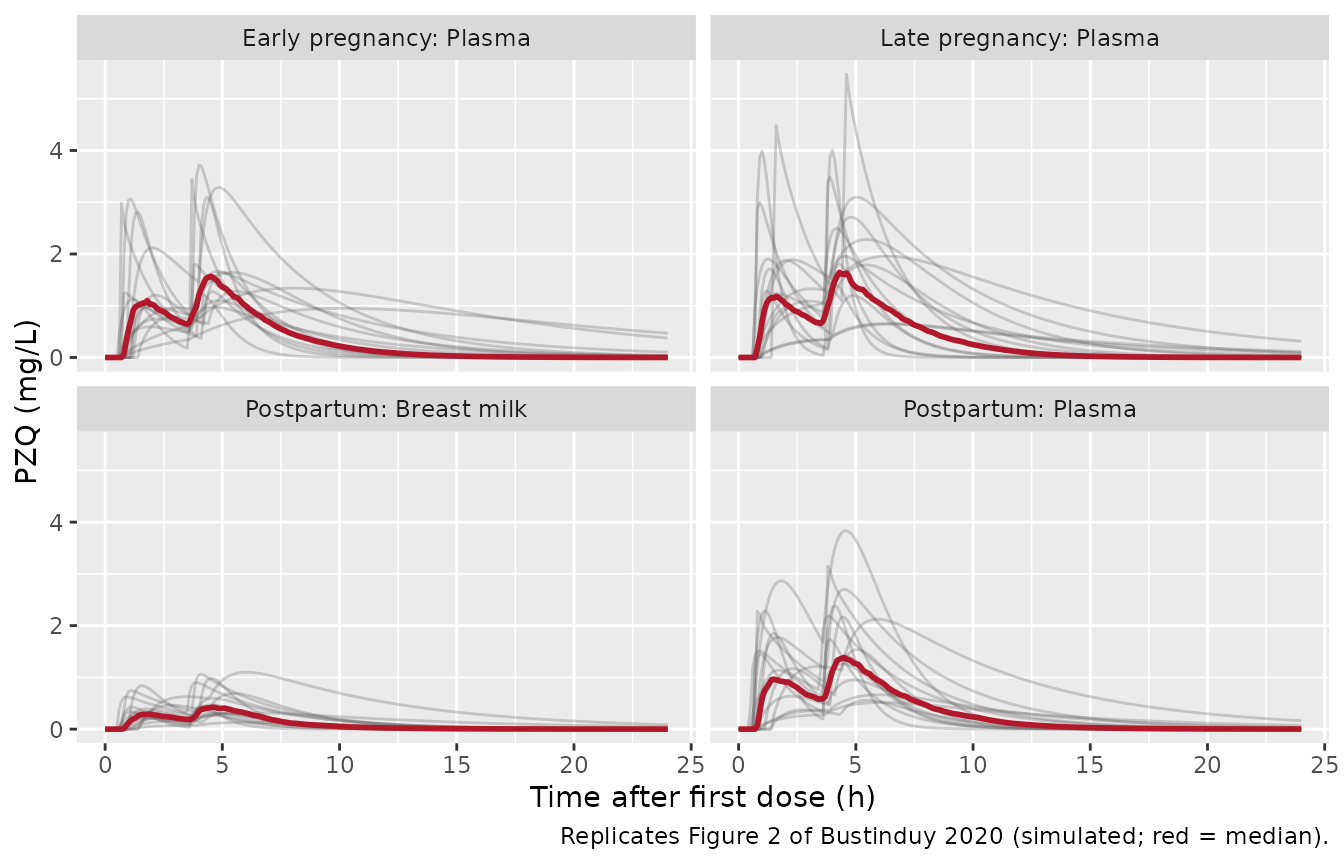
Median and individual plasma profiles by cohort, and milk in the postpartum cohort.

# Figure 7 of Bustinduy 2020: 1,000 simulated lactating women at the median
# weight of 47.9 kg; 5th/25th/50th/75th/95th centiles in plasma (A) and milk (B).
# 200 women are simulated here (the per-arm cohort cap).
ev7 <- dplyr::bind_rows(
  tidyr::crossing(id = 1:200, time = c(0, 3)) |>
    dplyr::mutate(amt = 30 * wt_ref, evid = 1L, cmt = "depot", dvid = NA_integer_),
  tidyr::crossing(id = 1:200, time = tgrid) |>
    dplyr::mutate(amt = NA_real_, evid = 0L, cmt = "central", dvid = 1L)
) |>
  dplyr::arrange(id, time, dplyr::desc(evid))
sim7 <- rxode2::rxSolve(mod, events = ev7) |> as.data.frame()

cent7 <- sim7 |>
  tidyr::pivot_longer(c(Cc, Cmilk), names_to = "matrix", values_to = "conc") |>
  dplyr::group_by(matrix, time) |>
  dplyr::summarise(
    p05 = stats::quantile(conc, 0.05), p25 = stats::quantile(conc, 0.25),
    p50 = stats::median(conc), p75 = stats::quantile(conc, 0.75),
    p95 = stats::quantile(conc, 0.95), .groups = "drop"
  ) |>
  dplyr::mutate(matrix = dplyr::recode(matrix, Cc = "A: plasma", Cmilk = "B: breast milk"))

ggplot(cent7, aes(time)) +
  geom_ribbon(aes(ymin = p05, ymax = p95), fill = "grey85") +
  geom_ribbon(aes(ymin = p25, ymax = p75), fill = "grey65") +
  geom_line(aes(y = p50), linewidth = 0.9) +
  facet_wrap(~matrix, ncol = 1) +
  labs(
    x = "Time (h)", y = "PZQ (mg/L)",
    caption = "Replicates Figure 7A-B of Bustinduy 2020 (5th-95th, 25th-75th centiles and median)."
  )

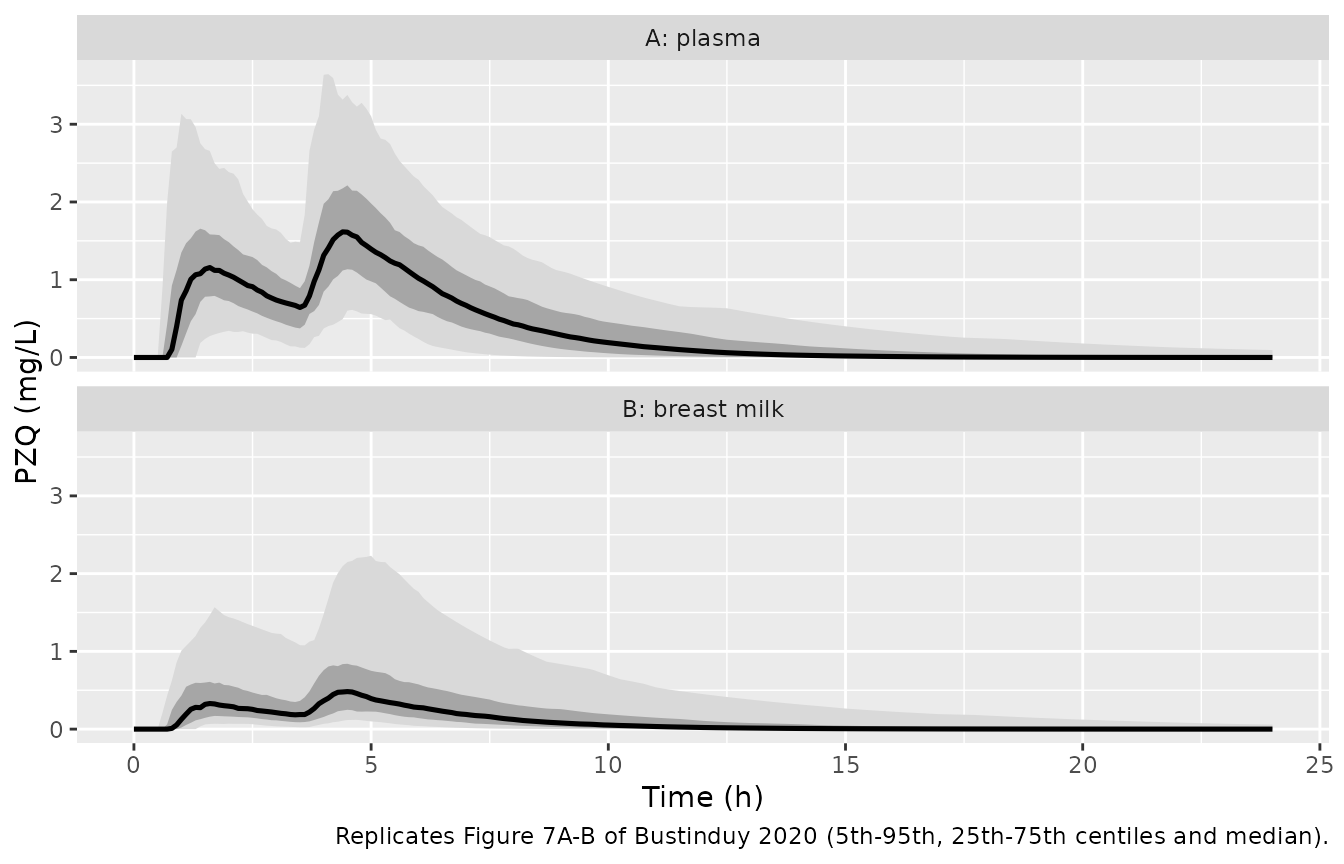
Monte Carlo centiles in 200 lactating women of 47.9 kg.

# Centiles at the second peak (t = 4.4 h), read from Figure 7A by the
# maintainers: about 0.65, 1.35, 1.85, 2.75 and 5.4 mg/L.
fig7_pub <- c(p05 = 0.65, p25 = 1.35, p50 = 1.85, p75 = 2.75, p95 = 5.4)
fig7_sim <- cent7 |>
  dplyr::filter(matrix == "A: plasma", abs(time - 4.4) < 1e-6) |>
  dplyr::select(p05:p95) |>
  unlist()
tibble::tibble(
  Centile = names(fig7_pub),
  `Figure 7A (digitised)` = fig7_pub,
  Simulated = round(fig7_sim, 2)
) |>
  knitr::kable(caption = "Plasma centiles at the second peak (4.4 h), mg/L.")

Plasma centiles at the second peak (4.4 h), mg/L.

Centile	Figure 7A (digitised)	Simulated
p05	0.65	0.49
p25	1.35	1.12
p50	1.85	1.62
p75	2.75	2.17
p95	5.40	3.32

# The simulated median sits within a factor of 1.6 of the digitised Figure 7A
# median. A mis-transcribed CL, V or dose unit moves it by a factor of several.
stopifnot(fig7_sim[["p50"]] > fig7_pub[["p50"]] / 1.6, fig7_sim[["p50"]] < fig7_pub[["p50"]] * 1.6)

The simulated centiles are narrower and lower than Figure 7A. That is expected for a log-normal model with independent etas: Pmetrics draws from the full NPAG covariance, including the r = 0.636 correlation between CL/F and V/F reported in the Results. The Figure 7C overlay puts most simulated women between 5 and 20 mgh/L in plasma and 2 and 10 mgh/L in milk. The cohort below falls in the same region.

PKNCA validation

dose_df <- events |>
  dplyr::filter(evid == 1) |>
  dplyr::select(id, time, amt, treatment)

# The ODE solver can undershoot zero by about its absolute tolerance on a
# decayed tail; PKNCA rejects negative concentrations (NaN AUC), so the tail is
# floored at zero. The minimum was asserted >= -1e-7 above.
conc_p <- sim |>
  dplyr::filter(!is.na(Cc)) |>
  dplyr::mutate(Cc = pmax(Cc, 0)) |>
  dplyr::select(id, time, Cc, treatment)
conc_m <- sim |>
  dplyr::filter(!is.na(Cmilk), treatment == "Postpartum") |>
  dplyr::mutate(Cmilk = pmax(Cmilk, 0)) |>
  dplyr::select(id, time, Cmilk, treatment)
stopifnot(all(tapply(conc_p$time, conc_p$id, min) == 0))

iv <- data.frame(start = 0, end = 24, cmax = TRUE, tmax = TRUE, auclast = TRUE)

nca_p <- PKNCA::pk.nca(PKNCA::PKNCAdata(
  PKNCA::PKNCAconc(conc_p, Cc ~ time | treatment + id),
  PKNCA::PKNCAdose(dose_df, amt ~ time | treatment + id),
  intervals = iv
)) |> as.data.frame()

nca_m <- PKNCA::pk.nca(PKNCA::PKNCAdata(
  PKNCA::PKNCAconc(conc_m, Cmilk ~ time | treatment + id),
  PKNCA::PKNCAdose(dplyr::filter(dose_df, treatment == "Postpartum"), amt ~ time | treatment + id),
  intervals = iv
)) |> as.data.frame()

stopifnot(
  !anyNA(nca_p$PPORRES[nca_p$PPTESTCD == "auclast"]),
  sum(nca_p$PPTESTCD == "auclast") == 3L * n_per_arm,
  !anyNA(nca_m$PPORRES[nca_m$PPTESTCD == "auclast"])
)

Comparison against published values

Figure 6D gives the posterior AUC0-24 by cohort as box plots. The maintainers digitised the medians as about 7.1 (early pregnancy), 11.8 (late pregnancy) and 11.2 (postpartum) mgh/L. The model has no cohort effect: the authors reported the early-pregnancy difference only as a post hoc comparison of Bayesian posteriors. The simulated cohorts therefore differ only through their weights. All three land near the pooled centre of about 9 mgh/L: above the early-pregnancy median and below the late-pregnancy and postpartum medians. Deviations of about 20-25% in either direction are the expected result of fitting one population to three cohorts whose posterior clearances differ by about 1.7-fold. They do not indicate a transcription error.

sim_med <- nca_p |>
  dplyr::filter(PPTESTCD %in% c("auclast", "cmax")) |>
  dplyr::group_by(treatment, PPTESTCD) |>
  dplyr::summarise(value = stats::median(PPORRES, na.rm = TRUE), .groups = "drop") |>
  tidyr::pivot_wider(names_from = PPTESTCD, values_from = value) |>
  dplyr::select(treatment, auclast)

published <- tibble::tribble(
  ~treatment, ~auclast,
  "Early pregnancy", 7.1,
  "Late pregnancy", 11.8,
  "Postpartum", 11.2
)

cmp <- nlmixr2lib::ncaComparisonTable(
  simulated = sim_med,
  reference = published,
  by = "treatment",
  units = c(auclast = "mg*h/L"),
  tolerance_pct = 20
)
knitr::kable(
  cmp,
  digits = 3,
  caption = paste(
    "Simulated median AUC0-24 vs the digitised Figure 6D medians.",
    "* differs from the reference by more than 20%."
  )
)

Simulated median AUC0-24 vs the digitised Figure 6D medians. * differs from the reference by more than 20%.

NCA parameter	treatment	Reference	Simulated	% diff
AUClast (mg*h/L)	Early pregnancy	7.1	8.87	+24.9%*
AUClast (mg*h/L)	Late pregnancy	11.8	9.49	-19.6%
AUClast (mg*h/L)	Postpartum	11.2	8.3	-25.9%*

# Pooled over all three cohorts, the simulated median AUC0-24 must sit near the
# pooled posterior centre (about 10 mg*h/L from Figure 6D). Centre-based gate.
pooled_auc <- stats::median(nca_p$PPORRES[nca_p$PPTESTCD == "auclast"])
stopifnot(pooled_auc > 10 / 1.5, pooled_auc < 10 * 1.5)

For breast milk the paper reports three posterior summaries over the 15 lactating women:

• mean average concentration 0.185 mg/L (AUC0-24 / 24);
• mean milk:plasma AUC0-24 ratio 0.36 (SD 0.13, range 0.19-0.55; printed as “AUCplasma:AUCbreast milk”, see Errata);
• “approximately 30%” partitioning in the Monte Carlo simulation.

milk_auc <- nca_m |>
  dplyr::filter(PPTESTCD == "auclast") |>
  dplyr::select(id, auc_milk = PPORRES)
plasma_auc_pp <- nca_p |>
  dplyr::filter(PPTESTCD == "auclast", treatment == "Postpartum") |>
  dplyr::select(id, auc_plasma = PPORRES)
milk_tab <- dplyr::inner_join(milk_auc, plasma_auc_pp, by = "id") |>
  dplyr::mutate(ratio = auc_milk / auc_plasma)
stopifnot(nrow(milk_tab) == n_per_arm)

milk_sum <- tibble::tibble(
  Quantity = c(
    "Mean milk Cavg0-24 (mg/L)", "Mean milk:plasma AUC0-24 ratio",
    "Median milk:plasma AUC0-24 ratio"
  ),
  Published = c(0.185, 0.36, 0.30),
  Simulated = c(
    mean(milk_tab$auc_milk) / 24, mean(milk_tab$ratio),
    stats::median(milk_tab$ratio)
  )
)
knitr::kable(milk_sum, digits = 3, caption = "Breast-milk exposure, postpartum cohort.")

Breast-milk exposure, postpartum cohort.

Quantity	Published	Simulated
Mean milk Cavg0-24 (mg/L)	0.185	0.218
Mean milk:plasma AUC0-24 ratio	0.360	0.580
Median milk:plasma AUC0-24 ratio	0.300	0.348

# Centre-based gates: the milk:plasma partition is set by (Kcb/Kbc)(Vc/Vb)
# and is 0.315 at typical values. A mis-transcribed milk parameter moves it
# by a factor.
stopifnot(
  stats::median(milk_tab$ratio) > 0.2, stats::median(milk_tab$ratio) < 0.45,
  mean(milk_tab$auc_milk) / 24 > 0.185 / 2, mean(milk_tab$auc_milk) / 24 < 0.185 * 2
)
# Figure 7C: the bulk of simulated women lie at 5-20 mg*h/L in plasma and
# 2-10 mg*h/L in milk. The cohort medians must fall in that region.
stopifnot(
  stats::median(milk_tab$auc_plasma) > 5, stats::median(milk_tab$auc_plasma) < 20,
  stats::median(milk_tab$auc_milk) > 2, stats::median(milk_tab$auc_milk) < 10
)

The simulated median ratio agrees with the paper. The simulated mean ratio is higher, because the independent log-normal etas on Kcb, Kbc, Vc and Vb give the ratio a long right tail. The posterior ratios of the 15 women spanned only 0.19-0.55.

The paper estimates infant intake by multiplying the average milk concentration by 0.15 L/kg/day: 0.185 x 0.15 = 0.028 mg/kg/day. The Abstract and Discussion instead quote 0.037 mg/kg/day. Either figure is roughly 1000-fold below the therapeutic 40-60 mg/kg.

Assumptions and deviations

• The Table 2 mean vector is used, not the median. See the mean-or-median section. The mean reproduces the population Monte Carlo (Figure 7) and the milk partitioning. The median reproduces the Results-text milk half-life and 24 h / 48 h concentrations for a single typical woman.
• IIV is a log-normal approximation to a non-parametric distribution. The Table 2 CV% (linear scale, confirmed above) is carried as omega^2 = log(CV^2 + 1). Covariances are not published, so the etas are independent. The one reported correlation (posterior CL/F and V/F, r = 0.636) is therefore missing, which is why the simulated Figure 7 spread differs from the published one. The Ka CV of 214% gives a very wide log-normal (omega^2 = 1.72), and the simulated absorption phase is correspondingly heterogeneous.
• No cohort (pregnancy-stage) effect. Posterior CL/F was higher in early pregnancy (P = 0.016) and AUC0-24 lower (P = 0.01). The authors reported this as a post hoc ANOVA on Bayesian posteriors and chose not to “further complicate the structural model”. No effect size is estimated inside the model, so none is encoded.
• The milk compartment is present for every woman. The model was fitted jointly to all 45 women, with milk observed only in the lactating cohort. Structurally, the reversible milk exchange acts as an extra distribution space in every simulated subject, as in the authors’ model.
• Weights are drawn from truncated normals with the Table 1 cohort means and SDs, over the roughly 36-63 kg range visible in Figure 5.
• Residual unexplained variability is fixed(0) for both outputs.

Errata and source-reporting gaps

• Methods equation (3) is printed XP(3) = Kcp x X(2) - Kcp x X(3). The return term must use Kpc, which is otherwise used only in eq. (2) and is an estimated Table 2 parameter.
• Methods equation (4) is printed XP(4) = -Kbc * X(4) - Kcb * X(2). The inflow must be positive (+ Kcb * X(2)), mirroring the - Kcb * X(2) loss in eq. (2). As printed, the milk amount would go negative and mass would not be conserved. The partition-identity check above confirms the corrected form.
• Output equation Y(1) = X(1) / Vc divides the gut amount. The plasma concentration is X(2) / Vc. Eq. (1) also prints “Bolas” for “Bolus”.
• Milk:plasma ratio label. The Results call the 0.36 figure “AUCplasma:AUCbreast milk”, but milk exposure is lower than plasma exposure (Figure 7C). The value is the milk:plasma ratio.
• Model compartment count. The paper calls its model “a standard 3-compartment PK model”, counting the gut as Pmetrics does. With the milk compartment, the fitted system has four states: two disposition compartments, a depot and a milk compartment.
• Residual error is unreported. Neither the Pmetrics assay-error polynomial nor a gamma/lambda term is given. The only supplemental item is Figure S1 (individual fits).