Model and source
- Citation: Han B, Xu N, Ma C, Ju G, Xi X, Qian C, Guo N, Liu X, Zhu X, Li C, Liu L (2025). Bridging Literature and Real-World Evidence: External Evaluation and Development of Fluoxetine Population Pharmacokinetics Model. Pharmaceutics 17(12):1516. doi:10.3390/pharmaceutics17121516.
- Description: Joint parent-metabolite population pharmacokinetic model for oral fluoxetine and its active metabolite norfluoxetine in 198 Chinese psychiatric adolescent and adult patients (146 female, 52 male; median age 17 years, range 12-56) receiving 20-60 mg once daily, developed from routine steady-state trough therapeutic-drug-monitoring records (Han 2025). Structural model: two connected one-compartment models – first-order absorption (Ka fixed at 0.3 1/h from the Panchaud 2011 literature model, because only trough samples were available) into a fluoxetine central compartment with first-order elimination, the whole of which (fraction metabolised fixed at 1) feeds a one-compartment norfluoxetine disposition with its own apparent clearance and apparent volume. Sex was the sole covariate retained by forward inclusion (p < 0.01) / backward elimination (p < 0.001): apparent fluoxetine clearance is 16.5% higher in males than in females, and the Table 4 typical values are the female-reference estimates. Between-subject variability is exponential on the apparent clearance of each analyte only; residual error is combined additive-plus-proportional, fitted separately for parent and metabolite. Because the fit used trough-only steady-state data, the apparent volumes (particularly the norfluoxetine volume, RSE 57%) are weakly identified and should be read as trough-reproducing rather than physiologic. The same paper externally evaluated the two previously published fluoxetine popPK models (Panchaud 2011, Wilens 2002) against this dataset and found both to underpredict at the population level.
- Article: https://doi.org/10.3390/pharmaceutics17121516
- Supplement (Tables S1-S4, Figures S1-S4): https://www.mdpi.com/article/10.3390/pharmaceutics17121516/s1
Han 2025 has three parts. It first assembles a repository of the published fluoxetine popPK models (two were found: Panchaud 2011 and Wilens 2002), then externally evaluates both against a Chinese therapeutic-drug-monitoring (TDM) dataset, and finally – because both literature models underpredicted at the population level – develops an original joint parent-metabolite model on that same dataset. Only the original joint model is packaged here. The two literature models are tabulated second-hand in Han 2025 Table 2; per the standing policy on secondary sources they should be extracted from their own primary publications rather than from this review’s summary table.
Population
The model was fitted to retrospective TDM records from 198 Chinese psychiatric patients treated with fluoxetine at Hunan Brain Hospital (the Second People’s Hospital of Hunan Province) between 2021 and 2024 (Han 2025 Table 1, “External dataset” row, and Sect. 3.3). The cohort was 73.7% female (146 of 198), with a median age of 17 years (range 12-56) and a median body weight of 59 kg (range 35.9-115). Roughly half the cohort was pediatric: 102 subjects were younger than 18 (median age 15, median weight 55 kg) and 92 were 18 or older (median age 21, median weight 59 kg). Daily doses ranged from 20 to 60 mg once daily with a median of 40 mg/day.
Sampling was trough-only – “All plasma samples were collected at steady state, prior to the next scheduled dose” (Sect. 2.3) – which is the single most important fact about this model, because it is why the absorption rate constant had to be fixed and why the apparent volumes are weakly identified. There were 241 fluoxetine and 241 norfluoxetine concentrations measured by LC-MS/MS with a lower limit of quantification of 1 ng/mL. The median observed fluoxetine trough was 140.97 ng/mL (range 7.43-979.93) and the median observed norfluoxetine trough was 129.2 ng/mL (range 9.6-490.41).
The same information is available programmatically via the model’s
population metadata:
str(readModelDb("Han_2025_fluoxetine")()$population, max.level = 1)
#> List of 16
#>  $ species       : chr "human"
#>  $ n_subjects    : int 198
#>  $ n_observations: int 482
#>  $ n_studies     : int 1
#>  $ age_range     : chr "12-56 years (median 17; Table 1)"
#>  $ age_median    : chr "17 years"
#>  $ weight_range  : chr "35.9-115 kg (median 59; Table 1)"
#>  $ weight_median : chr "59 kg"
#>  $ sex_female_pct: num 73.7
#>  $ race_ethnicity: Named num 100
#>   ..- attr(*, "names")= chr "Asian"
#>  $ disease_state : chr "Chinese psychiatric inpatients and outpatients treated with fluoxetine (predominantly depression; fluoxetine is"| __truncated__
#>  $ dose_range    : chr "20-60 mg once daily (Table 1 'External dataset' row). Note the paper is internally inconsistent about the upper"| __truncated__
#>  $ regions       : chr "China (Changsha, Hunan Province)"
#>  $ age_strata    : chr "Pediatric (< 18 years) n = 102, median age 15 (range 12-17), median weight 55 kg (range 35.9-96); adult (>= 18 "| __truncated__
#>  $ sampling      : chr "Trough-only: 'All plasma samples were collected at steady state, prior to the next scheduled dose' (Sect. 2.3);"| __truncated__
#>  $ notes         : chr "241 fluoxetine and 241 norfluoxetine plasma concentrations (482 observations total) from 198 subjects. Assay: v"| __truncated__
Source trace
The per-parameter origin is recorded as an in-file comment next to
each ini() entry in
inst/modeldb/specificDrugs/Han_2025_fluoxetine.R. The table
below collects them in one place for review. Every parameter value comes
from Han 2025 Table 4 (“The PK parameters with bootstrap results for the
final popPK model”); the structural statements come from the Methods and
Results text.
| Equation / parameter | Value | Source location |
|---|---|---|
| Structure: “two connected one-compartment models” | n/a | Sect. 3.5, first sentence |
d/dt(depot), first-order oral absorption |
n/a | Table 2 / Sect. 2.5 (every model in the repository is one-compartment with first-order absorption) |
d/dt(central_norfluox) fed by
fm * (cl / vc) * central
|
n/a | Table 4 abbreviations: “FM, the fraction of metabolism from fluoxetine to norfluoxetine” |
lka (Ka) |
0.3 1/h, fixed | Table 4 row “Ka (fixed) h-1”; rationale in Sect. 2.5 and Discussion (“Fixing ka (0.3 h-1) to a literature value was necessary given trough-only sampling”) |
lcl (fluoxetine CLP/F, female reference) |
2.91 L/h (RSE 23%) | Table 4 row “CL/F, L/h”, Fluoxetine block; bootstrap median 2.76 [1.53-4.13] |
lvc (fluoxetine VP/F) |
24.9 L (RSE 38%) | Table 4 row “V/F, L”, Fluoxetine block; bootstrap median 22.76 [9.06-38.48] |
fm (fraction metabolised) |
1, fixed | Table 4 row “FM (fixed)” |
lcl_norfluox (norfluoxetine CLM/F) |
3.24 L/h (RSE 20%) | Table 4 row “CL/F, L/h”, Norfluoxetine block; bootstrap median 3.06 [1.77-4.53]; also Sect. 3.5 text |
lvc_norfluox (norfluoxetine VM/F) |
1.52 L (RSE 57%) | Table 4 row “V/F, L”, Norfluoxetine block; bootstrap median 1.17 [0.67-1.98]; also Sect. 3.5 text |
e_sex_cl (male effect on CLP/F) |
0.165 (16.50%, RSE 44%) | Table 4 row “Sex effects on CL/F, %” and footnote 1:
CL/F,males = CL/F,females x (1 + 0.165), Females = 0, Males
= 1 |
etalcl |
CV 31.6% -> omega^2 = log(1 + 0.316^2) = 0.0951793 | Table 4 row “IIV CL/F, %”, Fluoxetine block (RSE 27%, eta-shrinkage 10%); exponential IIV per Sect. 2.5 |
etalcl_norfluox |
CV 20.9% -> omega^2 = log(1 + 0.209^2) = 0.0427539 | Table 4 row “IIV CL/F, %”, Norfluoxetine block (RSE 41%, eta-shrinkage 48%) |
propSd |
0.341 | Table 4 row “Prop.err.sd, %”, Fluoxetine block (34.1%, RSE 12%) |
addSd |
14.9 ng/mL | Table 4 row “Add.err.sd, ng/mL”, Fluoxetine block (RSE 49%) |
propSd_norfluox |
0.305 | Table 4 row “Prop.err.sd, %”, Norfluoxetine block (30.5%, RSE 16%) |
addSd_norfluox |
22.9 ng/mL | Table 4 row “Add.err.sd ng/mL”, Norfluoxetine block (RSE 31%) |
| Covariate search retaining only sex | n/a | Sect. 2.5 (forward p < 0.01, backward p < 0.001) and
Supplementary Table S3 (CL_SEX drop OFV 11.567, p =
0.000671; CL_WT “Failed”; CL_Age p =
0.180) |
Concentration unit conversion (1000 *) |
n/a | Table 1 LOQ “1 ng/mL”; Table 4 “Add.err.sd, ng/mL”; Sect. 3.6 target range in ng/mL |
| Validation target: PTA / trough table | n/a | Supplementary Table S4 |
Structural verification
Before simulating a cohort, three properties of the packaged model
are checked against closed-form arithmetic. These use
zeroRe() typical values, so both sides of each comparison
share the same parameters and the difference is pure numerical error –
tight bounds are appropriate here.
ui   <- rxode2::rxode2(readModelDb("Han_2025_fluoxetine"))
#> ℹ parameter labels from comments will be replaced by 'label()'
modz <- rxode2::zeroRe(ui)

tau <- 24
ev  <- rxode2::et(amt = 40, ii = tau, addl = 29, cmt = "depot") |>
  rxode2::et(seq(0, 30 * tau, by = 0.25))
d   <- as.data.frame(ev)
d$dvid <- ifelse(d$evid == 0, 1L, NA_integer_)
d$SEXF <- 1
s <- rxode2::rxSolve(modz, d, returnType = "data.frame")
#> ℹ omega/sigma items treated as zero: 'etalcl', 'etalcl_norfluox'

# 1. Steady-state trough of the parent against the analytic one-compartment
#    oral multiple-dose solution.
cl <- 2.91; vc <- 24.9; ka <- 0.3; kel <- cl / vc; dose <- 40
cf <- 1000 * (dose * ka) / (vc * (ka - kel)) *
  (exp(-kel * tau) / (1 - exp(-kel * tau)) -
     exp(-ka * tau) / (1 - exp(-ka * tau)))
obs_trough <- s$Cc[nrow(s)]

# 2. Mass balance over one steady-state interval. With fm fixed at 1 the whole
#    dose is eliminated as parent and re-formed as metabolite, so
#    cl * AUCtau(parent) == clm * AUCtau(metabolite) == dose.
ss   <- s[s$time >= 29 * tau & s$time <= 30 * tau, ]
trap <- function(x, y) sum(diff(x) * (head(y, -1) + tail(y, -1)) / 2)
auc_p <- trap(ss$time, ss$Cc) / 1000
auc_m <- trap(ss$time, ss$Cc_norfluox) / 1000

# 3. The sex effect must be exactly the +16.5% of the Table 4 footnote.
dm <- d; dm$SEXF <- 0
sm <- rxode2::rxSolve(modz, dm, returnType = "data.frame")
#> ℹ omega/sigma items treated as zero: 'etalcl', 'etalcl_norfluox'

structural <- tibble::tibble(
  Check = c("SS parent trough vs analytic solution (ng/mL)",
            "cl * AUCtau(fluoxetine) vs dose (mg)",
            "clm * AUCtau(norfluoxetine) vs dose (mg)",
            "male:female CL ratio"),
  Model     = c(obs_trough, cl * auc_p, 3.24 * auc_m, sm$cl[1] / s$cl[1]),
  Reference = c(cf, dose, dose, 1.165)
) |>
  mutate(`Difference (%)` = 100 * (Model - Reference) / Reference)
knitr::kable(structural, digits = 5,
caption = "Closed-form structural checks on typical values.")| Check | Model | Reference | Difference (%) |
|---|---|---|---|
| SS parent trough vs analytic solution (ng/mL) | 167.54967 | 167.5497 | 0.00000 |
| cl * AUCtau(fluoxetine) vs dose (mg) | 39.99270 | 40.0000 | -0.01826 |
| clm * AUCtau(norfluoxetine) vs dose (mg) | 39.99996 | 40.0000 | -0.00010 |
| male:female CL ratio | 1.16500 | 1.1650 | 0.00000 |
Virtual cohort
Han 2025 simulated 1000 virtual patients per scenario for six once-daily doses (10-60 mg) in each sex, and reported the resulting steady-state trough distributions and probabilities of target attainment in Supplementary Table S4. That table is reproduced below.
Three choices differ from the paper’s Monte Carlo design:
- 200 subjects per arm, not 1000 (the package-wide cohort cap). Twelve arms (2 sexes x 6 dose levels) give 2400 subjects in total.
-
A deterministic quantile lattice instead of random
draws. The only random effects in this model are the two
clearance etas, so each arm’s etas are placed on an evenly spaced normal
quantile lattice rather than sampled. The metabolite eta is paired to
the parent eta through a fixed coprime stride permutation, which keeps
the two approximately independent while involving no random number
generator at all. The cohort is therefore identical on every machine and
thread count, which an
rxSetSeed()-based approach cannot guarantee (rxode2 partitions its RNG streams per solver thread). - 10 daily doses rather than 30. With an apparent half-life of about 6 h the accumulation is essentially complete after two days; the chunk below proves steady state was reached rather than assuming it.
The omega values are read back out of the packaged model rather than re-typed, so this chunk fails loudly if the model file’s IIV ever changes.
om <- diag(ui$omega)
stopifnot(setequal(names(om), c("etalcl", "etalcl_norfluox")))

n_arm  <- 200L
ndose  <- 10L
t_last <- (ndose - 1L) * tau      # start of the final dosing interval

lat  <- (seq_len(n_arm) - 0.5) / n_arm
perm <- ((seq_len(n_arm) - 1L) * 97L) %% n_arm + 1L   # 97 is coprime to 200
eta_cl  <- qnorm(lat, sd = sqrt(om[["etalcl"]]))
eta_clm <- qnorm(lat, sd = sqrt(om[["etalcl_norfluox"]]))[perm]
stopifnot(abs(cor(eta_cl, eta_clm)) < 0.1)   # the pairing is near-independent

arms <- tidyr::expand_grid(sexf = c(1L, 0L),
                           dose = c(10, 20, 30, 40, 50, 60)) |>
  mutate(sex       = ifelse(sexf == 1L, "Female", "Male"),
         arm       = sprintf("%s %g mg", sex, dose),
         id_offset = (row_number() - 1L) * n_arm)

# `subject_ids` selects which lattice points appear in an arm, so the same
# builder serves both the full 200/arm trough cohort and the 50/arm subset
# used for NCA.
make_arm <- function(sexf, dose, id_offset, arm, sex, obs_t, subject_ids) {
  e <- rxode2::et(amt = dose, ii = tau, addl = ndose - 1L, cmt = "depot") |>
    rxode2::et(obs_t) |>
    rxode2::et(id = subject_ids)
  e <- as.data.frame(e)
  e$dvid <- ifelse(e$evid == 0, 1L, NA_integer_)
  k      <- e$id
  e$id   <- e$id + id_offset
  e$SEXF <- sexf
  e$etalcl          <- eta_cl[k]
  e$etalcl_norfluox <- eta_clm[k]
  e$arm  <- arm
  e$sex  <- sex
  e$dose <- dose
  e
}

build_events <- function(obs_t, subject_ids) {
  do.call(rbind, Map(make_arm, arms$sexf, arms$dose, arms$id_offset,
                     arms$arm, arms$sex,
                     MoreArgs = list(obs_t = obs_t, subject_ids = subject_ids)))
}

# Trough cohort: the two interval-boundary troughs only. Their equality is
# the steady-state proof.
events_trough <- build_events(c(t_last, t_last + tau), seq_len(n_arm))
stopifnot(dplyr::n_distinct(events_trough$id) == n_arm * nrow(arms))
Simulation
The etas are supplied as data columns against a zeroRe()
model: the model’s own random-effect simulation is switched off and each
subject’s eta is read from the event table, which is how the
deterministic lattice is injected.
sim_trough <- rxode2::rxSolve(modz, events_trough,
                              keep = c("arm", "sex", "dose"),
                              returnType = "data.frame")
#> ℹ omega/sigma items treated as zero: 'etalcl', 'etalcl_norfluox'
#> Warning: multi-subject simulation without without 'omega'

# Steady state: the trough at the start of the final interval must equal the
# trough at its end, for every subject and both analytes.
b0 <- sim_trough[abs(sim_trough$time - t_last) < 1e-6, ]
b1 <- sim_trough[abs(sim_trough$time - (t_last + tau)) < 1e-6, ]
stopifnot(nrow(b0) == nrow(b1),
          max(abs(b1$Cc - b0$Cc) / b0$Cc) < 1e-3,
          max(abs(b1$Cc_norfluox - b0$Cc_norfluox) / b0$Cc_norfluox) < 1e-3)

trough <- b1 |>
  transmute(id, arm, sex, dose,
            Fluoxetine      = Cc,
            Norfluoxetine   = Cc_norfluox,
            `Active moiety` = Cc + Cc_norfluox)
stopifnot(nrow(trough) == n_arm * nrow(arms), !anyNA(trough))
Note that Cc and Cc_norfluox are the
individual predictions – they carry between-subject variability but no
residual error. That is the right comparator for Table S4: Han 2025’s
simulated trough quartiles are far narrower than a
residual-error-inclusive simulation would produce, so their Monte Carlo
evidently propagated IIV only.
Replicate Supplementary Table S4
Table S4 reports, for each sex x dose x analyte combination, the probability of attaining the therapeutic window and the median, first and third quartiles of the steady-state trough concentration. All 36 rows are transcribed below and compared on the concentration quantiles.
published <- tibble::tribble(
  ~sex, ~dose, ~analyte, ~pub_pta, ~pub_med, ~pub_q1, ~pub_q3,
  "Female", 10, "Active moiety",  24.8,  83.72,  54.61, 119.72,
  "Female", 20, "Active moiety",  69.7, 167.44, 109.23, 239.43,
  "Female", 30, "Active moiety",  77.2, 251.16, 163.84, 359.15,
  "Female", 40, "Active moiety",  70.9, 334.88, 218.45, 478.87,
  "Female", 50, "Active moiety",  60.3, 418.60, 273.06, 598.58,
  "Female", 60, "Active moiety",  47.0, 502.32, 327.68, 718.30,
  "Male",   10, "Active moiety",  12.1,  62.14,  38.79,  92.17,
  "Male",   20, "Active moiety",  52.7, 124.28,  77.57, 184.35,
  "Male",   30, "Active moiety",  69.7, 186.42, 116.36, 276.52,
  "Male",   40, "Active moiety",  73.9, 248.56, 155.15, 368.69,
  "Male",   50, "Active moiety",  68.5, 310.70, 193.94, 460.86,
  "Male",   60, "Active moiety",  64.1, 372.84, 232.72, 553.04,
  "Female", 10, "Fluoxetine",     11.9,  42.99,  26.36,  68.11,
  "Female", 20, "Fluoxetine",     44.3,  85.97,  52.72, 136.22,
  "Female", 30, "Fluoxetine",     58.3, 128.96,  79.09, 204.33,
  "Female", 40, "Fluoxetine",     60.2, 171.95, 105.45, 272.43,
  "Female", 50, "Fluoxetine",     54.6, 214.94, 131.81, 340.54,
  "Female", 60, "Fluoxetine",     49.4, 257.92, 158.17, 408.65,
  "Male",   10, "Fluoxetine",      5.7,  29.40,  17.14,  48.83,
  "Male",   20, "Fluoxetine",     27.2,  58.81,  34.27,  97.66,
  "Male",   30, "Fluoxetine",     45.2,  88.21,  51.41, 146.49,
  "Male",   40, "Fluoxetine",     53.1, 117.61,  68.54, 195.31,
  "Male",   50, "Fluoxetine",     57.7, 147.02,  85.68, 244.14,
  "Male",   60, "Fluoxetine",     55.2, 176.42, 102.82, 292.97,
  "Female", 10, "Norfluoxetine",   5.7,  39.45,  27.98,  53.29,
  "Female", 20, "Norfluoxetine",  58.0,  78.90,  55.97, 106.58,
  "Female", 30, "Norfluoxetine",  81.6, 118.35,  83.95, 159.87,
  "Female", 40, "Norfluoxetine",  82.1, 157.80, 111.93, 213.16,
  "Female", 50, "Norfluoxetine",  69.8, 197.25, 139.91, 266.45,
  "Female", 60, "Norfluoxetine",  55.5, 236.70, 167.90, 319.74,
  "Male",   10, "Norfluoxetine",   2.3,  31.85,  21.45,  44.57,
  "Male",   20, "Norfluoxetine",  39.9,  63.70,  42.89,  89.15,
  "Male",   30, "Norfluoxetine",  67.5,  95.55,  64.34, 133.72,
  "Male",   40, "Norfluoxetine",  78.5, 127.41,  85.79, 178.29,
  "Male",   50, "Norfluoxetine",  74.4, 159.26, 107.24, 222.87,
  "Male",   60, "Norfluoxetine",  67.1, 191.11, 128.68, 267.44
)

simulated <- trough |>
  tidyr::pivot_longer(c(Fluoxetine, Norfluoxetine, `Active moiety`),
                      names_to = "analyte", values_to = "conc") |>
  group_by(sex, dose, analyte) |>
  summarise(sim_pta = 100 * mean(conc >= 120 & conc <= 500),
            sim_med = median(conc),
            sim_q1  = quantile(conc, 0.25),
            sim_q3  = quantile(conc, 0.75),
            .groups = "drop")

s4 <- published |>
  left_join(simulated, by = c("sex", "dose", "analyte")) |>
  mutate(d_med = 100 * (sim_med - pub_med) / pub_med,
         d_q1  = 100 * (sim_q1  - pub_q1)  / pub_q1,
         d_q3  = 100 * (sim_q3  - pub_q3)  / pub_q3,
         d_pta = sim_pta - pub_pta) |>
  arrange(analyte, sex, dose)
stopifnot(nrow(s4) == 36L, !anyNA(s4))

s4 |>
  transmute(Analyte = analyte, Sex = sex, `Dose (mg)` = dose,
            `Median published` = pub_med, `Median simulated` = round(sim_med, 2),
            `Median diff (%)`  = round(d_med, 1),
            `Q1 published`     = pub_q1, `Q1 simulated` = round(sim_q1, 2),
            `Q1 diff (%)`      = round(d_q1, 1),
            `Q3 published`     = pub_q3, `Q3 simulated` = round(sim_q3, 2),
            `Q3 diff (%)`      = round(d_q3, 1)) |>
  knitr::kable(
    caption = paste("Replicates Supplementary Table S4 of Han 2025:",
                    "steady-state trough concentrations (ng/mL) by analyte,",
"sex and dose."))| Analyte | Sex | Dose (mg) | Median published | Median simulated | Median diff (%) | Q1 published | Q1 simulated | Q1 diff (%) | Q3 published | Q3 simulated | Q3 diff (%) |
|---|---|---|---|---|---|---|---|---|---|---|---|
| Active moiety | Female | 10 | 83.72 | 81.97 | -2.1 | 54.61 | 55.23 | 1.1 | 119.72 | 123.43 | 3.1 |
| Active moiety | Female | 20 | 167.44 | 163.95 | -2.1 | 109.23 | 110.46 | 1.1 | 239.43 | 246.87 | 3.1 |
| Active moiety | Female | 30 | 251.16 | 245.92 | -2.1 | 163.84 | 165.69 | 1.1 | 359.15 | 370.30 | 3.1 |
| Active moiety | Female | 40 | 334.88 | 327.90 | -2.1 | 218.45 | 220.92 | 1.1 | 478.87 | 493.73 | 3.1 |
| Active moiety | Female | 50 | 418.60 | 409.87 | -2.1 | 273.06 | 276.15 | 1.1 | 598.58 | 617.17 | 3.1 |
| Active moiety | Female | 60 | 502.32 | 491.85 | -2.1 | 327.68 | 331.38 | 1.1 | 718.30 | 740.60 | 3.1 |
| Active moiety | Male | 10 | 62.14 | 60.53 | -2.6 | 38.79 | 39.09 | 0.8 | 92.17 | 95.35 | 3.5 |
| Active moiety | Male | 20 | 124.28 | 121.06 | -2.6 | 77.57 | 78.18 | 0.8 | 184.35 | 190.70 | 3.4 |
| Active moiety | Male | 30 | 186.42 | 181.58 | -2.6 | 116.36 | 117.27 | 0.8 | 276.52 | 286.06 | 3.4 |
| Active moiety | Male | 40 | 248.56 | 242.11 | -2.6 | 155.15 | 156.36 | 0.8 | 368.69 | 381.41 | 3.4 |
| Active moiety | Male | 50 | 310.70 | 302.64 | -2.6 | 193.94 | 195.45 | 0.8 | 460.86 | 476.76 | 3.5 |
| Active moiety | Male | 60 | 372.84 | 363.17 | -2.6 | 232.72 | 234.55 | 0.8 | 553.04 | 572.11 | 3.4 |
| Fluoxetine | Female | 10 | 42.99 | 41.89 | -2.6 | 26.36 | 24.72 | -6.2 | 68.11 | 66.49 | -2.4 |
| Fluoxetine | Female | 20 | 85.97 | 83.78 | -2.6 | 52.72 | 49.43 | -6.2 | 136.22 | 132.97 | -2.4 |
| Fluoxetine | Female | 30 | 128.96 | 125.66 | -2.6 | 79.09 | 74.15 | -6.2 | 204.33 | 199.46 | -2.4 |
| Fluoxetine | Female | 40 | 171.95 | 167.55 | -2.6 | 105.45 | 98.86 | -6.2 | 272.43 | 265.94 | -2.4 |
| Fluoxetine | Female | 50 | 214.94 | 209.44 | -2.6 | 131.81 | 123.58 | -6.2 | 340.54 | 332.43 | -2.4 |
| Fluoxetine | Female | 60 | 257.92 | 251.33 | -2.6 | 158.17 | 148.29 | -6.2 | 408.65 | 398.91 | -2.4 |
| Fluoxetine | Male | 10 | 29.40 | 28.57 | -2.8 | 17.14 | 15.96 | -6.9 | 48.83 | 47.55 | -2.6 |
| Fluoxetine | Male | 20 | 58.81 | 57.15 | -2.8 | 34.27 | 31.92 | -6.9 | 97.66 | 95.10 | -2.6 |
| Fluoxetine | Male | 30 | 88.21 | 85.72 | -2.8 | 51.41 | 47.88 | -6.9 | 146.49 | 142.65 | -2.6 |
| Fluoxetine | Male | 40 | 117.61 | 114.30 | -2.8 | 68.54 | 63.84 | -6.9 | 195.31 | 190.20 | -2.6 |
| Fluoxetine | Male | 50 | 147.02 | 142.87 | -2.8 | 85.68 | 79.80 | -6.9 | 244.14 | 237.76 | -2.6 |
| Fluoxetine | Male | 60 | 176.42 | 171.44 | -2.8 | 102.82 | 95.76 | -6.9 | 292.97 | 285.31 | -2.6 |
| Norfluoxetine | Female | 10 | 39.45 | 39.23 | -0.6 | 27.98 | 25.14 | -10.1 | 53.29 | 52.81 | -0.9 |
| Norfluoxetine | Female | 20 | 78.90 | 78.46 | -0.6 | 55.97 | 50.28 | -10.2 | 106.58 | 105.61 | -0.9 |
| Norfluoxetine | Female | 30 | 118.35 | 117.69 | -0.6 | 83.95 | 75.42 | -10.2 | 159.87 | 158.42 | -0.9 |
| Norfluoxetine | Female | 40 | 157.80 | 156.93 | -0.6 | 111.93 | 100.57 | -10.2 | 213.16 | 211.22 | -0.9 |
| Norfluoxetine | Female | 50 | 197.25 | 196.16 | -0.6 | 139.91 | 125.71 | -10.2 | 266.45 | 264.03 | -0.9 |
| Norfluoxetine | Female | 60 | 236.70 | 235.39 | -0.6 | 167.90 | 150.85 | -10.2 | 319.74 | 316.83 | -0.9 |
| Norfluoxetine | Male | 10 | 31.85 | 31.67 | -0.6 | 21.45 | 19.29 | -10.1 | 44.57 | 46.25 | 3.8 |
| Norfluoxetine | Male | 20 | 63.70 | 63.34 | -0.6 | 42.89 | 38.58 | -10.0 | 89.15 | 92.50 | 3.8 |
| Norfluoxetine | Male | 30 | 95.55 | 95.01 | -0.6 | 64.34 | 57.87 | -10.0 | 133.72 | 138.76 | 3.8 |
| Norfluoxetine | Male | 40 | 127.41 | 126.69 | -0.6 | 85.79 | 77.17 | -10.1 | 178.29 | 185.01 | 3.8 |
| Norfluoxetine | Male | 50 | 159.26 | 158.36 | -0.6 | 107.24 | 96.46 | -10.1 | 222.87 | 231.26 | 3.8 |
| Norfluoxetine | Male | 60 | 191.11 | 190.03 | -0.6 | 128.68 | 115.75 | -10.0 | 267.44 | 277.51 | 3.8 |
The whole 36-row table is reproduced with a central bias of a couple of percent. That bias is the size expected from Monte Carlo error alone: the standard error of a median from 1000 log-normal draws with this spread is around 3%, and the published medians are exactly dose-proportional within each sex x analyte block, which shows one drawn cohort was scaled across all six dose levels rather than six independent draws. A single common offset per block is therefore the signature of one Monte Carlo draw, not of a transcription error.
The assertions below are written on the centre and on robust quantiles of the discrepancy rather than on any single extreme row.
stopifnot(
  # Centre: a mis-transcribed clearance, dose or unit would shift the whole
  # distribution by tens of percent and blow this instantly.
  abs(median(s4$d_med)) < 5,
  abs(median(s4$d_q1))  < 9,
  abs(median(s4$d_q3))  < 9,
  # Envelope: robust to which arms land in the tails.
  quantile(abs(s4$d_med), 0.9) < 8,
  quantile(abs(s4$d_q1),  0.9) < 15,
  quantile(abs(s4$d_q3),  0.9) < 12
)
Probability of target attainment
The 120-500 ng/mL therapeutic window is defined by Han 2025 only for the active moiety – Sect. 2.6: “The proportion of individuals meeting pre-defined therapeutic exposure targets (fluoxetine plus norfluoxetine 120-500 ng/mL)”. Table S4’s “Target” column names the analyte, not a concentration range, and the paper never states a numeric window for fluoxetine or norfluoxetine alone. The PTA comparison is therefore restricted to the active-moiety rows.
That restriction is not a convenience. The published per-analyte PTA
values are arithmetically incompatible with the 120-500 window given
their own published quartiles: a distribution whose median is below 120
cannot place more than half its mass inside [120, 500], and
one whose third quartile is below 120 cannot place more than a quarter
there. The check below finds the offending rows from the published
numbers alone, with no simulation involved.
impossible <- published |>
  filter(analyte != "Active moiety",
         (pub_med < 120 & pub_pta > 50) | (pub_q3 < 120 & pub_pta > 25)) |>
  transmute(Analyte = analyte, Sex = sex, `Dose (mg)` = dose,
            `Published median` = pub_med, `Published Q3` = pub_q3,
            `Published PTA (%)` = pub_pta,
            `Maximum attainable PTA (%)` = ifelse(pub_q3 < 120, 25, 50))
knitr::kable(
  impossible,
  caption = paste("Published Table S4 rows whose PTA cannot be against the",
"120-500 ng/mL window, given the same row's own quartiles."))| Analyte | Sex | Dose (mg) | Published median | Published Q3 | Published PTA (%) | Maximum attainable PTA (%) |
|---|---|---|---|---|---|---|
| Fluoxetine | Male | 20 | 58.81 | 97.66 | 27.2 | 25 |
| Fluoxetine | Male | 40 | 117.61 | 195.31 | 53.1 | 50 |
| Norfluoxetine | Female | 20 | 78.90 | 106.58 | 58.0 | 25 |
| Norfluoxetine | Female | 30 | 118.35 | 159.87 | 81.6 | 50 |
| Norfluoxetine | Male | 20 | 63.70 | 89.15 | 39.9 | 25 |
| Norfluoxetine | Male | 30 | 95.55 | 133.72 | 67.5 | 50 |
For the active moiety, where the target is unambiguous, the simulated and published PTA agree to within three percentage points at every dose in both sexes.
pta_act <- s4 |> filter(analyte == "Active moiety")
pta_act |>
  transmute(Sex = sex, `Dose (mg)` = dose,
            `PTA published (%)` = pub_pta,
            `PTA simulated (%)` = round(sim_pta, 1),
            `Difference (pct pt)` = round(d_pta, 1)) |>
  knitr::kable(caption = paste("Active-moiety probability of attaining",
"120-500 ng/mL: published versus simulated."))| Sex | Dose (mg) | PTA published (%) | PTA simulated (%) | Difference (pct pt) |
|---|---|---|---|---|
| Female | 10 | 24.8 | 25.5 | 0.7 |
| Female | 20 | 69.7 | 68.0 | -1.7 |
| Female | 30 | 77.2 | 76.5 | -0.7 |
| Female | 40 | 70.9 | 71.5 | 0.6 |
| Female | 50 | 60.3 | 59.5 | -0.8 |
| Female | 60 | 47.0 | 49.5 | 2.5 |
| Male | 10 | 12.1 | 13.5 | 1.4 |
| Male | 20 | 52.7 | 50.5 | -2.2 |
| Male | 30 | 69.7 | 72.5 | 2.8 |
| Male | 40 | 73.9 | 71.0 | -2.9 |
| Male | 50 | 68.5 | 68.0 | -0.5 |
| Male | 60 | 64.1 | 63.5 | -0.6 |
Replicate Figure 5
Figure 5 of Han 2025 plots the probability of attaining the active-moiety target against daily dose, separately for each sex.
pta_act |>
  select(sex, dose, Published = pub_pta, Simulated = sim_pta) |>
  tidyr::pivot_longer(c(Published, Simulated),
                      names_to = "source", values_to = "pta") |>
  ggplot(aes(dose, pta, colour = sex, linetype = source, shape = source)) +
  geom_hline(yintercept = 70, colour = "grey60", linetype = "dotted") +
  geom_line() +
  geom_point() +
  scale_x_continuous(breaks = c(10, 20, 30, 40, 50, 60)) +
  labs(x = "Daily dose (mg QD)",
       y = "PTA for active moiety 120-500 ng/mL (%)",
       colour = "Sex", linetype = NULL, shape = NULL,
       title = "Figure 5 - probability of target attainment",
       caption = "Replicates Figure 5 / Supplementary Table S4 of Han 2025.")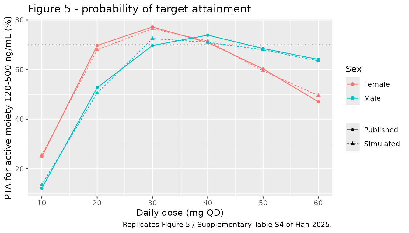
Sect. 3.6 reads this figure as “when administered to females at a dose of 20-40 mg/day, the PTA exceeded 70%, and when administered to males at a dose of 30-50 mg/day, the PTA also exceeded 70%”. That prose rounds its own table: Table S4 puts female 20 mg at 69.7% and male 50 mg at 68.5%, both just under 70. The assertions below therefore gate the directional content of the claim – a broad, sex-shifted plateau of high attainment, with females plateauing one dose level lower than males – rather than the literal 70% threshold.
f <- pta_act |> filter(sex == "Female") |> arrange(dose)
m <- pta_act |> filter(sex == "Male")   |> arrange(dose)
stopifnot(
  # Females: the 20-40 mg plateau.
  all(f$sim_pta[f$dose %in% c(20, 30, 40)] > 65),
  # Males: the 30-50 mg plateau.
  all(m$sim_pta[m$dose %in% c(30, 40, 50)] > 65),
  # 10 mg is clearly subtherapeutic in both sexes.
  f$sim_pta[f$dose == 10] < 35, m$sim_pta[m$dose == 10] < 25,
  # The female plateau starts a dose level lower than the male one.
  f$sim_pta[f$dose == 20] > m$sim_pta[m$dose == 20],
  # Females sit higher on the exposure axis at every dose, because male
  # clearance is 16.5% higher.
  all(f$sim_med > m$sim_med),
  # Attainment falls away again at the top of the range for females, the
  # paper's basis for capping them at 30-40 mg (Sect. 3.6, Conclusions).
  f$sim_pta[f$dose == 60] < f$sim_pta[f$dose == 30]
)
PKNCA validation
NCA is run over the final steady-state dosing interval, with time re-expressed relative to the start of that interval and the dose group carried into the PKNCA formula so per-arm results can be compared. A dense concentration grid is needed for Cmax and Tmax, so this uses an evenly spaced 50-subject subset of each arm’s lattice (600 subjects) rather than the full trough cohort.
nca_ids     <- seq(2L, n_arm, by = 4L)          # 50 evenly spaced lattice points
obs_t       <- seq(t_last, t_last + tau, by = 0.5)
events_nca  <- build_events(obs_t, nca_ids)
sim_nca     <- rxode2::rxSolve(modz, events_nca, keep = c("arm", "sex", "dose"),
                               returnType = "data.frame")
#> ℹ omega/sigma items treated as zero: 'etalcl', 'etalcl_norfluox'
#> Warning: multi-subject simulation without without 'omega'
stopifnot(dplyr::n_distinct(sim_nca$id) == length(nca_ids) * nrow(arms))
conc_data <- sim_nca |>
  dplyr::filter(!is.na(Cc)) |>
  dplyr::transmute(id, arm, sex, dose, time = time - t_last, conc = Cc)
# The NCA interval starts at a dose, so a time-zero record exists by
# construction; assert it rather than assuming it.
stopifnot(sum(conc_data$time == 0) == dplyr::n_distinct(conc_data$id),
          all(dplyr::count(conc_data, id)$n == length(obs_t)))

dose_data <- sim_nca |>
  dplyr::distinct(id, arm, sex, dose) |>
  dplyr::mutate(time = 0, amt_mg = dose)

o_conc <- PKNCA::PKNCAconc(conc_data, conc ~ time | id / arm)
o_dose <- PKNCA::PKNCAdose(dose_data, amt_mg ~ time | id)
intervals <- data.frame(start = 0, end = tau,
                        cmax = TRUE, tmax = TRUE, auclast = TRUE,
                        clast.obs = TRUE, half.life = TRUE)
res_nca <- suppressWarnings(
  PKNCA::pk.nca(PKNCA::PKNCAdata(o_conc, o_dose, intervals = intervals)))

nca <- as.data.frame(res_nca) |>
  dplyr::filter(PPTESTCD %in% c("cmax", "tmax", "auclast", "clast.obs",
                                "half.life")) |>
  dplyr::select(id, PPTESTCD, PPORRES) |>
  tidyr::pivot_wider(names_from = PPTESTCD, values_from = PPORRES) |>
  dplyr::mutate(id = as.integer(as.character(id))) |>
  dplyr::left_join(dplyr::distinct(sim_nca, id, arm, sex, dose), by = "id")
stopifnot(nrow(nca) == length(nca_ids) * nrow(arms), !anyNA(nca$auclast))
The steady-state interval AUC is itself a closed-form check: because
the model is linear and dosing is at steady state, CL/F
must equal dose / AUCtau exactly for every individual. This
compares the NCA result against each subject’s own clearance, so the
only difference is trapezoidal integration error and a tight bound is
appropriate.
cl_check <- nca |>
  dplyr::left_join(dplyr::distinct(events_nca, id, etalcl), by = "id") |>
  dplyr::mutate(
    cl_model = 2.91 * exp(etalcl) * (1 + 0.165 * (sex == "Male")),
    cl_nca   = dose / (auclast / 1000),
    rel_pct  = 100 * (cl_nca - cl_model) / cl_model)
knitr::kable(
  cl_check |>
    dplyr::group_by(Sex = sex) |>
    dplyr::summarise(`Median CL/F from AUCtau (L/h)` = round(median(cl_nca), 4),
                     `Median model CL/F (L/h)` = round(median(cl_model), 4),
                     `Max |difference| (%)` = round(max(abs(rel_pct)), 4),
                     .groups = "drop"),
  caption = paste("CL/F recovered from the steady-state AUCtau versus each",
"subject's model clearance."))| Sex | Median CL/F from AUCtau (L/h) | Median model CL/F (L/h) | Max |difference| (%) |
|---|---|---|---|
| Female | 2.9069 | 2.9045 | 0.1765 |
| Male | 3.3871 | 3.3837 | 0.2065 |
Comparison against published NCA
Han 2025 reports no NCA parameters – it is a trough-only TDM
analysis, so there is no published Cmax, Tmax, AUC or half-life to
compare against. The one exposure metric it does publish is the
steady-state trough, which corresponds to clast.obs over
the final dosing interval (the concentration at the end of the interval;
PKNCA’s cmin over the same interval would return the trough
at its start). The comparison below is therefore against the
median fluoxetine trough of Supplementary Table S4 for each sex and
dose.
sim_nca_wide <- nca |>
  dplyr::group_by(sex, dose) |>
  dplyr::summarise(clast.obs = median(clast.obs), .groups = "drop") |>
  dplyr::mutate(dose = paste(dose, "mg"))

ref_nca_wide <- published |>
  dplyr::filter(analyte == "Fluoxetine") |>
  dplyr::transmute(sex, dose = paste(dose, "mg"), clast.obs = pub_med)

cmp <- nlmixr2lib::ncaComparisonTable(
  simulated = sim_nca_wide,
  reference = ref_nca_wide,
  by        = c("sex", "dose"),
  units     = c(clast.obs = "ng/mL"),
  tolerance_pct = 20)
cmp
#>    NCA parameter    sex  dose Reference Simulated % diff
#> 1  Clast (ng/mL) Female 10 mg        43      42.1  -2.1%
#> 2  Clast (ng/mL) Female 20 mg        86      84.2  -2.1%
#> 3  Clast (ng/mL) Female 30 mg       129       126  -2.1%
#> 4  Clast (ng/mL) Female 40 mg       172       168  -2.1%
#> 5  Clast (ng/mL) Female 50 mg       215       210  -2.1%
#> 6  Clast (ng/mL) Female 60 mg       258       253  -2.1%
#> 7  Clast (ng/mL)   Male 10 mg      29.4      28.7  -2.3%
#> 8  Clast (ng/mL)   Male 20 mg      58.8      57.4  -2.3%
#> 9  Clast (ng/mL)   Male 30 mg      88.2      86.2  -2.3%
#> 10 Clast (ng/mL)   Male 40 mg       118       115  -2.3%
#> 11 Clast (ng/mL)   Male 50 mg       147       144  -2.3%
#> 12 Clast (ng/mL)   Male 60 mg       176       172  -2.3%
For completeness, the other NCA parameters the simulation produces over the steady-state interval are summarised below. They have no published counterpart, but they make the shape of the model explicit – in particular the roughly 6 h apparent terminal half-life, which is far shorter than fluoxetine’s literature half-life of 4-6 days and is discussed under Assumptions below.
nca |>
  dplyr::group_by(Sex = sex, `Dose (mg)` = dose) |>
  dplyr::summarise(`Cmax (ng/mL)`     = round(median(cmax), 1),
                   `Tmax (h)`         = round(median(tmax), 2),
                   `AUCtau (ng*h/mL)` = round(median(auclast), 0),
                   `Ctrough (ng/mL)`  = round(median(clast.obs), 1),
                   `t1/2 (h)`         = round(median(half.life), 2),
                   .groups = "drop") |>
  knitr::kable(caption = paste("Simulated steady-state NCA parameters for",
"fluoxetine, by arm."))| Sex | Dose (mg) | Cmax (ng/mL) | Tmax (h) | AUCtau (ng*h/mL) | Ctrough (ng/mL) | t1/2 (h) |
|---|---|---|---|---|---|---|
| Female | 10 | 243.8 | 5.0 | 3440 | 42.1 | 6.20 |
| Female | 20 | 487.5 | 5.0 | 6881 | 84.2 | 6.20 |
| Female | 30 | 731.3 | 5.0 | 10321 | 126.3 | 6.20 |
| Female | 40 | 975.0 | 5.0 | 13761 | 168.3 | 6.20 |
| Female | 50 | 1218.8 | 5.0 | 17201 | 210.4 | 6.20 |
| Female | 60 | 1462.6 | 5.0 | 20642 | 252.5 | 6.20 |
| Male | 10 | 223.7 | 4.5 | 2953 | 28.7 | 5.36 |
| Male | 20 | 447.4 | 4.5 | 5905 | 57.4 | 5.36 |
| Male | 30 | 671.2 | 4.5 | 8858 | 86.2 | 5.36 |
| Male | 40 | 894.9 | 4.5 | 11810 | 114.9 | 5.36 |
| Male | 50 | 1118.6 | 4.5 | 14763 | 143.6 | 5.36 |
| Male | 60 | 1342.3 | 4.5 | 17716 | 172.3 | 5.36 |
Assumptions and deviations
Only the original joint model is packaged. Han 2025 also tabulates the Panchaud 2011 and Wilens 2002 fluoxetine models (Table 2) and externally evaluates them (Table 3). Those are other authors’ models reported second-hand; extracting them from this paper’s summary table would lose the covariate encoding, reference values and error-model detail that only the primary publications carry. They should be extracted from their own sources.
IIV scale. Table 4 reports IIV as a percent without stating whether it is
100 * omegaor100 * sqrt(exp(omega^2) - 1). The model file uses the exact log-normal identityomega^2 = log(1 + CV^2). For IIVs this small the two conventions differ by under 3% in omega (0.3086 versus 0.3160 for the parent), and the Table S4 quartiles reproduced above cannot distinguish them. They do decisively rule out the two other readings: taking 31.6% to mean the variance itself, or the variance expressed as a percent, produces interquartile ranges roughly twice as wide and roughly a third as wide respectively as the published ones.Residual error is excluded from the Table S4 comparison. The published trough quartiles are matched by an IIV-only simulation; adding the additive-plus-proportional residual error would widen the interquartile range well past the published values. The model file carries the full residual error as published, and
sim(rather thanCc) should be used when a residual-error-inclusive simulation is wanted.The published per-analyte PTA columns cannot be reproduced, and are internally inconsistent. Table S4 gives a PTA for fluoxetine and for norfluoxetine as well as for the active moiety, but the paper defines a numeric target only for the active moiety (120-500 ng/mL, Sect. 2.6), and Table S4’s “Target” column holds analyte names rather than concentration ranges. Six of the 24 per-analyte rows are impossible against the 120-500 window given their own quartiles – female 30 mg norfluoxetine, for instance, reports a median of 118.35 ng/mL (below the lower bound, so at most half the cohort can attain the window) alongside a PTA of 81.6%; female 20 mg norfluoxetine reports Q3 = 106.58 (so at most a quarter can attain it) alongside a PTA of 58.0%. The
pta-published-consistencychunk enumerates all six. The most likely explanation is an analyte-specific target the paper does not report. This vignette therefore compares PTA only for the active moiety, where agreement is within three percentage points at every dose, and compares the fluoxetine and norfluoxetine rows on their quantiles – which do reproduce. This is a reporting gap in the source, not a discrepancy in the packaged model.The apparent volumes are not physiologic.
V/F = 24.9 Limplies an apparent terminal half-life of about 5.9 h, whereas fluoxetine’s literature half-life is 4-6 days (Han 2025 Introduction). This is a direct consequence of fitting a one-compartment model to trough-only data: the volume is whatever reproduces the 24-hour trough, not a distribution volume.VM/F = 1.52 L(RSE 57%) is more extreme still, implying a norfluoxetine half-life of about 20 minutes, so the metabolite is effectively formation-rate-limited in this model. Neither value should be reused outside a trough-prediction context. The Discussion acknowledges the underlying limitation (“all samples were collected at trough concentrations, which may limit the robustness of model development, particularly with respect to accurately characterizing the absorption rate”).FMfixed at 1 with no molar correction. Table 4 fixes the fraction of fluoxetine metabolised to norfluoxetine at 1, and the paper applies no molecular-weight conversion between the two species (fluoxetine 309.33, norfluoxetine 295.31 g/mol). BecauseCLM/FandVM/Fare apparent parameters estimated conditional onFM = 1, any true fraction below 1 and the 4.5% mass difference are both absorbed into them; the model is reproduced exactly as published.Sex stored under the canonical
SEXF. Han 2025 encodes sex as a male indicator with female as the reference (Table 4 footnote 1). The canonical covariate column isSEXF(1 = female), so the effect is applied as(1 + e_sex_cl * (1 - SEXF)), which preserves the published female-referenceCL/F = 2.91 L/hand the published +16.5% male increment verbatim. This matches the construction already used byBajaj_2017_nivolumab.R,Wada_2023_sparsentan.RandLi_2012_clozapine.R.No covariate on the metabolite. Supplementary Table S3 shows that sex on metabolite clearance (
CLM_SEX) reached p = 0.045 in the first forward cycle – above the p < 0.01 inclusion threshold – and p = 0.239 in the second, so it was never included. Weight failed to converge on every parameter it was tested on (CL_WTandCLM_WT, both “Failed”), and age was non-significant throughout.WTandAGEare therefore recorded in the model file’scovariatesDataExcludedrather thancovariateData.Cohort size and sampling design. 200 subjects per arm on a deterministic quantile lattice, versus the paper’s 1000 randomly drawn subjects per scenario, and 10 daily doses rather than 30 (steady state is asserted, not assumed). The lattice removes Monte Carlo noise from this side of the comparison entirely, but it truncates the extreme tails, which slightly compresses the simulated quartiles relative to a random draw – visible as the systematically low first quartile in the Table S4 comparison.
Internal inconsistencies in the source. Two, neither of which affects the model: Sect. 3.3 gives the cohort dose range as 20-40 mg/day while Table 1 and the Discussion both give 20-60 mg/day; and the pediatric (n = 102) and adult (n = 92) strata sum to 194 rather than the 198 subjects reported for the whole cohort. Both are recorded in the model file’s
populationmetadata.Table 4 compound labels. In the published Table 4 the “Compounds” column labels the norfluoxetine
CL/FandV/Frows “Fluoxetine”. The Sect. 3.5 text is unambiguous that 3.24 L/h and 1.52 L belong to norfluoxetine (“For norfluoxetine, CLM/F was 3.24 L/h (RSE: 20%), and VM/F was 1.52 L (RSE: 57%)”), and the bootstrap column aligns those values with the Norfluoxetine rows, so the text was followed.