Emicizumab (Retout 2020)
Source:vignettes/articles/Retout_2020_emicizumab.Rmd
Retout_2020_emicizumab.RmdModel and source
- Citation: Retout S, Schmitt C, Petry C, Mercier F, Frey N. Population Pharmacokinetic Analysis and Exploratory Exposure-Bleeding Rate Relationship of Emicizumab in Adult and Pediatric Persons with Hemophilia A. Clin Pharmacokinet. 2020;59(12):1611-1625. doi:10.1007/s40262-020-00904-z
- Description: One-compartment population PK model with first-order subcutaneous absorption and first-order elimination (no lag time) for emicizumab, a bispecific anti-FIXa/FX humanized monoclonal antibody, in adult, adolescent and pediatric (1 year and older) persons with hemophilia A with or without factor VIII inhibitors (Retout 2020; phase I/II + HAVEN 1-4). Body weight (power, 70 kg) and albumin (linear, 45 g/L) on CL/F, body weight (power) and Black race (fractional) on V/F, and a linear decline of the apparent bioavailability F above 30 years of age.
- Article: doi:10.1007/s40262-020-00904-z (open access, CC BY-NC 4.0)
- Trial registries: HAVEN 1 NCT02622321, HAVEN 2 NCT02795767, HAVEN 3 NCT02847637, HAVEN 4 NCT03020160, Japanese phase I/II JapicCTI-121934 / JapicCTI-132195.
Emicizumab is a humanized bispecific IgG4 antibody that bridges activated factor IX and factor X, replacing the cofactor function of the missing activated factor VIII in persons with hemophilia A (PwHA). Retout 2020 pooled the phase I/II study and the four phase III HAVEN studies into one population PK analysis. The final model is a linear one-compartment model with first-order subcutaneous absorption and elimination and no lag time. Its covariates are body weight and albumin on CL/F, body weight and Black race on V/F, and an age-dependent apparent bioavailability F that declines linearly above 30 years.
The earlier analysis of the phase I/II data alone is packaged
separately as Yoneyama_2017_emicizumab. Retout 2020’s
exposure-bleeding analysis (Section 2.4, Figure 6) is a descriptive
comparison of estimated average concentrations across
annualized-bleeding-rate categories. It fits no model, so nothing from
it is packaged here.
Population
The analysis population was 389 PwHA with or without factor VIII (FVIII) inhibitors from five studies (Retout 2020 Tables 1-3): the Japanese phase I/II study (n = 18), HAVEN 1 (n = 112), HAVEN 2 (pediatric, n = 63), HAVEN 3 (n = 148) and HAVEN 4 (n = 48). Age ranged from 1.22 to 77.0 years (median 30.0) and body weight from 9.50 to 156 kg (median 69.1). Median albumin was 45.0 g/L. The population was 62.7% White, 8.0% Black, 22.9% Asian (including Japanese) and 6.4% other or unknown, and 49.9% had FVIII inhibitors. Most PwHA received 3 mg/kg QW for 4 weeks followed by 1.5 mg/kg QW (75.1%); 12.6% received the 3 mg/kg Q2W maintenance and 12.3% the 6 mg/kg Q4W maintenance. The paper does not tabulate sex. Hemophilia A is X-linked, so the cohort is expected to be male.
The same information is available programmatically via
readModelDb("Retout_2020_emicizumab")()$population.
Source trace
Every ini() value carries an in-file comment pointing to
its source. The table below collects them.
| Equation / parameter | Value | Source location |
|---|---|---|
lka |
log(0.536) 1/day | Table 4, KA |
lcl |
log(0.272) L/day | Table 4, CL/F (BW 70 kg, ALB 45 g/L, age <= 30 years) |
lvc |
log(10.4) L | Table 4, V/F |
e_wt_cl |
0.911 | Table 4, ‘Effect of BW on CL/F’ |
e_alb_cl |
0.0157 | Table 4, ‘Effect of ALB on CL/F’; sign from the Section 3.1 CL/F equation |
e_wt_vc |
1.00 | Table 4, ‘Effect of BW on V/F’ |
e_race_black_vc |
-0.215 | Table 4, ‘Effect of Black on V/F’ |
e_age_fdepot |
0.00651 | Table 4, ‘Effect of AGE>30 years on F’; sign from the Section 3.1 F equation |
etalcl, etalvc, etalka
|
0.079152, 0.064927, 0.422400 | Table 4, BPV 28.7%, 25.9%, 72.5% CV;
omega^2 = log(1 + CV^2)
|
cov(etalcl, etalvc) |
0.015556 | Table 4, correlation CL/F-V/F 0.217 |
cov(etalcl, etalka) |
-0.062352 | Table 4, correlation CL/F-KA -0.341 |
cov(etalvc, etalka) |
0 | Not reported in Table 4 |
addSd |
0.025 ug/mL (fixed) | Table 4, sigma1 additive; Section 3.1 (half the phase I/II LLOQ) |
propSd |
0.146 | Table 4, sigma2 proportional 14.6% |
cl, vc, fdepot equations |
n/a | Section 3.1 covariate equations |
| One-compartment ODE, first-order absorption, no lag | n/a | Section 3.1, first paragraph |
Closed-form checks against the paper’s reference patient
Retout 2020 reports steady-state predictions for a reference PwHA who
is White or Asian, 30 years old, 70 kg and has albumin 45 g/L, dosed at
1.5 mg/kg QW (Section 3.2). For a linear model,
Cav,SS = F * Dose / (CL/F * tau) exactly, so each of the
paper’s statements is a direct test of the packaged parameters and
equation signs.
mod <- readModelDb("Retout_2020_emicizumab")
ui <- rxode2::rxode(mod)
#> ℹ parameter labels from comments will be replaced by 'label()'
th <- setNames(ui$iniDf$est, ui$iniDf$name)

typ_cl <- function(WT, ALB) {
  exp(th[["lcl"]]) * (WT / 70)^th[["e_wt_cl"]] * (1 - th[["e_alb_cl"]] * (ALB - 45))
}
typ_f <- function(AGE) {
  1 - th[["e_age_fdepot"]] * (AGE > 30) * (AGE - 30)
}
typ_cav <- function(WT, ALB, AGE, mgkg = 1.5, tau = 7) {
  typ_f(AGE) * mgkg * WT / (typ_cl(WT, ALB) * tau)
}

cav_ref <- typ_cav(70, 45, 30)
closed <- tibble::tribble(
  ~Claim, ~Paper, ~Packaged,
  "Cav,SS reference PwHA (ug/mL)", 55.1, cav_ref,
  "Cav,SS at ALB 33 g/L (ug/mL)", 46.4, typ_cav(70, 33, 30),
  "Cav,SS at ALB 57 g/L (ug/mL)", 68.0, typ_cav(70, 57, 30),
  "Exposure change at 77 years (%)", -31, 100 * (typ_cav(70, 45, 77) / cav_ref - 1),
  "CL/F change at 9 kg (%)", -85, 100 * ((9 / 70)^th[["e_wt_cl"]] - 1),
  "CL/F change at 156 kg (%)", 108, 100 * ((156 / 70)^th[["e_wt_cl"]] - 1),
  "V/F change at 9 kg (%)", -87, 100 * ((9 / 70)^th[["e_wt_vc"]] - 1),
  "V/F change at 156 kg (%)", 123, 100 * ((156 / 70)^th[["e_wt_vc"]] - 1),
  "V/F change, Black race (%)", -22, 100 * th[["e_race_black_vc"]],
  "Typical absorption half-life (day)", 1.27, log(2) / exp(th[["lka"]])
)
knitr::kable(closed, digits = 2, caption = "Reference-patient statements in Retout 2020 (Sections 3.1, 3.2 and 4, Figure 2 caption) against the packaged model. The half-life row compares the typical value with the Table 5 median.")| Claim | Paper | Packaged |
|---|---|---|
| Cav,SS reference PwHA (ug/mL) | 55.10 | 55.15 |
| Cav,SS at ALB 33 g/L (ug/mL) | 46.40 | 46.40 |
| Cav,SS at ALB 57 g/L (ug/mL) | 68.00 | 67.95 |
| Exposure change at 77 years (%) | -31.00 | -30.60 |
| CL/F change at 9 kg (%) | -85.00 | -84.57 |
| CL/F change at 156 kg (%) | 108.00 | 107.52 |
| V/F change at 9 kg (%) | -87.00 | -87.14 |
| V/F change at 156 kg (%) | 123.00 | 122.86 |
| V/F change, Black race (%) | -22.00 | -21.50 |
| Typical absorption half-life (day) | 1.27 | 1.29 |
# All ten are deterministic functions of the packaged parameters. Each
# published value is printed to 2-3 significant figures, so agreement to
# within the printed rounding is the test. A sign error on the albumin or
# age term moves the corresponding row by 20-40%.
stopifnot(
  abs(cav_ref - 55.1) < 0.1,
  abs(typ_cav(70, 33, 30) - 46.4) < 0.1,
  abs(typ_cav(70, 57, 30) - 68.0) < 0.1,
  abs(100 * (typ_cav(70, 45, 77) / cav_ref - 1) - (-31)) < 0.5,
  abs(100 * ((9 / 70)^th[["e_wt_cl"]] - 1) - (-85)) < 0.5,
  abs(100 * ((156 / 70)^th[["e_wt_cl"]] - 1) - 108) < 0.5,
  abs(100 * ((9 / 70)^th[["e_wt_vc"]] - 1) - (-87)) < 0.5,
  abs(100 * ((156 / 70)^th[["e_wt_vc"]] - 1) - 123) < 0.5,
  abs(log(2) / exp(th[["lka"]]) - 1.27) < 0.05
)
The albumin rows show which sign is right. Table 4 prints the albumin
coefficient as +1.57e-2. Under the Methods’ generic form
(1 + theta * (ALB - 45)), that would give 68.0 ug/mL at 33
g/L and 46.4 ug/mL at 57 g/L, the reverse of what the paper reports. The
Section 3.1 equation (1 - 0.0157 * (ALB - 45)) reproduces
both published values, so clearance falls as albumin rises. The age
coefficient works the same way: Table 4 prints +6.51e-3,
and the equation’s minus sign gives the published 31% exposure loss at
77 years.
Replicate Figure 4: covariate impact at steady state
Figure 4 of Retout 2020 shows typical-value steady-state profiles over one 1.5 mg/kg QW dosing interval for 12 covariate combinations. The paper simulated steady state directly. Here the regimen is run for two years (3 mg/kg QW loading for 4 weeks, then 1.5 mg/kg QW) and the final interval is plotted. At the typical 26.5-day half-life, the remaining gap from true steady state is below 1e-8.
# One subject per row of `subj`. The regimen is 3 mg/kg QW x 4 loading, then
# maintenance `mgkg` every `tau` days up to day 756; observations every 6 h
# over the final interval [756 - tau, 756] (6 h is the paper's step, Section 2.3).
t_end <- 28 + 728

make_events <- function(subj, mgkg, tau, obs_times) {
  maint <- seq(28, t_end - tau, by = tau)
  dose <- tidyr::crossing(
    subj,
    tibble::tibble(time = c(0, 7, 14, 21, maint), mgkg_dose = c(rep(3, 4), rep(mgkg, length(maint))))
  ) |>
    dplyr::mutate(amt = mgkg_dose * WT, evid = 1L, cmt = "depot") |>
    dplyr::select(-mgkg_dose)
  obs <- tidyr::crossing(subj, tibble::tibble(time = obs_times)) |>
    dplyr::mutate(amt = 0, evid = 0L, cmt = "central")
  dplyr::bind_rows(dose, obs) |>
    dplyr::arrange(id, time, dplyr::desc(evid)) |>
    as.data.frame()
}

fig4_subj <- tibble::tribble(
  ~panel, ~label, ~WT, ~AGE, ~ALB, ~RACE_BLACK,
  "Body weight", "31 kg - 8 y", 31, 8, 45, 0,
  "Body weight", "70 kg - 30 y", 70, 30, 45, 0,
  "Body weight", "156 kg - 30 y", 156, 30, 45, 0,
  "Age", "6 y - 20 kg", 20, 6, 45, 0,
  "Age", "12 y - 40 kg", 40, 12, 45, 0,
  "Age", "30 y - 70 kg", 70, 30, 45, 0,
  "Age", "50 y - 70 kg", 70, 50, 45, 0,
  "Age", "77 y - 70 kg", 70, 77, 45, 0,
  "Race", "White or Asian", 70, 30, 45, 0,
  "Race", "Black", 70, 30, 45, 1,
  "Albumin", "ALB = 33 g/L", 70, 30, 33, 0,
  "Albumin", "ALB = 45 g/L", 70, 30, 45, 0,
  "Albumin", "ALB = 57 g/L", 70, 30, 57, 0
) |>
  dplyr::mutate(id = dplyr::row_number())

ev_fig4 <- make_events(
  dplyr::select(fig4_subj, id, WT, AGE, ALB, RACE_BLACK),
  mgkg = 1.5, tau = 7, obs_times = seq(t_end - 7, t_end, by = 0.25)
)
mod_typ <- rxode2::zeroRe(mod)
#> ℹ parameter labels from comments will be replaced by 'label()'

# Every solve below is on the zero-variance model. Where per-subject etas are
# supplied as event-table columns, rxode2 warns that a multi-subject solve
# has no omega, which is intended here. Muffle that one warning only.
muffle_no_omega <- function(w) {
  if (grepl("without 'omega'", conditionMessage(w), fixed = TRUE)) {
    invokeRestart("muffleWarning")
  }
}
solve_typ <- function(events, ...) {
  withCallingHandlers(
    rxode2::rxSolve(mod_typ, events = events, ...),
    warning = muffle_no_omega
  )
}

sim_fig4 <- solve_typ(ev_fig4, rtol = 1e-10, atol = 1e-12) |>
  as.data.frame() |>
  dplyr::left_join(dplyr::select(fig4_subj, id, panel, label), by = "id") |>
  dplyr::mutate(
    tad = time - (t_end - 7),
    label = factor(label, levels = unique(fig4_subj$label))
  )
#> ℹ omega/sigma items treated as zero: 'etalka', 'etalcl', 'etalvc'
ggplot(sim_fig4, aes(tad, Cc)) +
  geom_line(colour = "red", linewidth = 1) +
  facet_wrap(~ panel + label, ncol = 5) +
  coord_cartesian(ylim = c(0, 75)) +
  labs(
    x = "Time over a dosing interval at steady state (day)",
    y = "Predicted emicizumab concentration (ug/mL)",
    caption = "Replicates Figure 4 of Retout 2020 (1.5 mg/kg QW, typical values)."
  ) +
  theme_bw()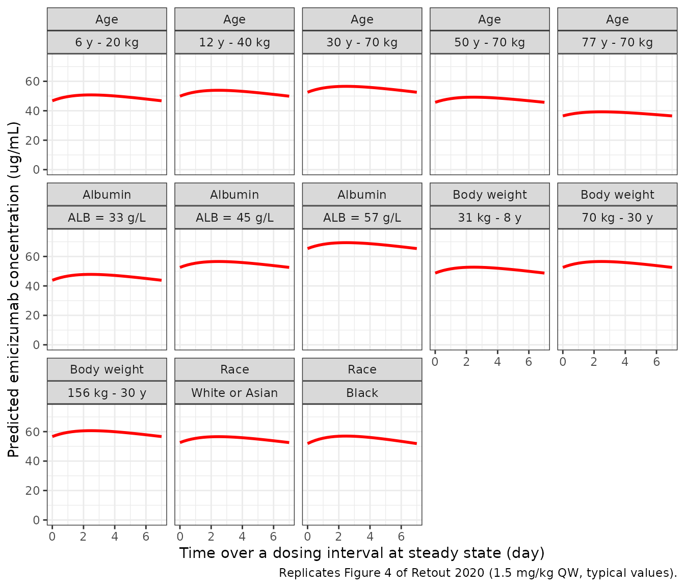
fig4_sum <- sim_fig4 |>
  dplyr::group_by(id, label) |>
  dplyr::summarise(Cmax = max(Cc), Ctrough = min(Cc), .groups = "drop")
knitr::kable(fig4_sum, digits = 1, caption = "Typical steady-state Cmax and Ctrough per Figure 4 scenario.")| id | label | Cmax | Ctrough |
|---|---|---|---|
| 1 | 31 kg - 8 y | 52.7 | 48.7 |
| 2 | 70 kg - 30 y | 56.6 | 52.6 |
| 3 | 156 kg - 30 y | 60.7 | 56.7 |
| 4 | 6 y - 20 kg | 50.8 | 46.8 |
| 5 | 12 y - 40 kg | 53.9 | 49.9 |
| 6 | 30 y - 70 kg | 56.6 | 52.6 |
| 7 | 50 y - 70 kg | 49.2 | 45.7 |
| 8 | 77 y - 70 kg | 39.3 | 36.5 |
| 9 | White or Asian | 56.6 | 52.6 |
| 10 | Black | 57.0 | 51.9 |
| 11 | ALB = 33 g/L | 47.8 | 43.8 |
| 12 | ALB = 45 g/L | 56.6 | 52.6 |
| 13 | ALB = 57 g/L | 69.4 | 65.4 |
race <- fig4_sum |> dplyr::filter(label %in% c("White or Asian", "Black"))
race_trough <- 100 * (race$Ctrough[race$label == "Black"] / race$Ctrough[race$label == "White or Asian"] - 1)
race_peak <- 100 * (race$Cmax[race$label == "Black"] / race$Cmax[race$label == "White or Asian"] - 1)
c(race_trough_pct = race_trough, race_peak_pct = race_peak)
#> race_trough_pct   race_peak_pct
#>      -1.3195546       0.7003509

# Section 3.2: in Black PwHA, Ctrough,SS falls by less than 2% and Cmax,SS
# rises by less than 1% relative to the White/Asian reference. Both are
# typical-value solves (no random draws); measured -1.32% and +0.70%. The
# lower bounds catch a race effect that is too small: -0.0215 gives -0.13%
# and +0.07%, which the paper's "< 2%" / "< 1%" alone would accept.
stopifnot(race_trough < -1, race_trough > -2, race_peak > 0.5, race_peak < 1)
The simulated profiles match Figure 4 as read by eye. The weight panels peak at 52.7, 56.6 and 60.7 ug/mL (Figure 4: about 52.5, 56.5 and 60.5); the 77-year panel peaks at 39.3 ug/mL (about 39); and the 33 / 57 g/L albumin panels peak at 47.8 and 69.4 ug/mL (about 48 and 69.5).
Virtual cohort for Table 5
Table 5 of Retout 2020 summarises steady-state exposure from the individual PK parameters of 381 PwHA under each maintenance regimen. The individual data are not public. The virtual cohort below approximates the analysis population from Tables 2-3: 16% pediatric (HAVEN 2: age 1.2-15.7 years, median weight 22.6 kg) and 84% adolescent/adult (median age about 33 years, median weight about 74 kg). Albumin is centred on 45 g/L and 8% of the cohort is Black.
Between-subject random effects are drawn in R from the packaged
omega matrix and passed to a zeroRe() model as
per-subject columns. The same 200 individuals (same covariates and
random effects) therefore receive each of the three regimens, as in
Table 5. This reproduces the paper’s result that Cav,SS is
identical across regimens. The cohort is also identical on every
machine, because no draw depends on rxode2’s thread-partitioned RNG.
set.seed(20200605)

# Draw from a lognormal, rejecting and redrawing outside [lo, hi] so the band
# limits are definitions, not clamps that pile subjects on the boundary.
rtrunc_lnorm <- function(n, median, sdlog, lo, hi) {
  x <- stats::rlnorm(n, log(median), sdlog)
  bad <- x < lo | x > hi
  while (any(bad)) {
    x[bad] <- stats::rlnorm(sum(bad), log(median), sdlog)
    bad <- x < lo | x > hi
  }
  x
}
rtrunc_norm <- function(n, mean, sd, lo, hi) {
  x <- stats::rnorm(n, mean, sd)
  bad <- x < lo | x > hi
  while (any(bad)) {
    x[bad] <- stats::rnorm(sum(bad), mean, sd)
    bad <- x < lo | x > hi
  }
  x
}

# Approximate median weight-for-age (10 kg at 1 year, 23 kg at 7 years,
# 46 kg at 12 years) with 15% lognormal spread, redrawn into the HAVEN 2
# weight range 9.5-63 kg.
rped_wt <- function(age) {
  med <- 10 * exp(0.139 * (age - 1))
  x <- med * exp(stats::rnorm(length(age), 0, 0.15))
  bad <- x < 9.5 | x > 63
  while (any(bad)) {
    x[bad] <- med[bad] * exp(stats::rnorm(sum(bad), 0, 0.15))
    bad <- x < 9.5 | x > 63
  }
  x
}

make_cohort <- function(n_ped, n_adult, id_offset = 0L) {
  age_ped <- stats::runif(n_ped, 1, 12)
  wt_ped <- rped_wt(age_ped)
  age_ad <- rtrunc_lnorm(n_adult, 33, 0.40, 12, 77)
  wt_ad <- rtrunc_lnorm(n_adult, 74, 0.20, 40, 156)
  n <- n_ped + n_adult
  tibble::tibble(
    id = id_offset + seq_len(n),
    age_group = rep(c("1 to <12 years", ">=12 years"), c(n_ped, n_adult)),
    AGE = c(age_ped, age_ad),
    WT = c(wt_ped, wt_ad),
    ALB = rtrunc_norm(n, 45, 3.5, 33, 57),
    RACE_BLACK = stats::rbinom(n, 1, 0.08)
  )
}

# Random effects from the packaged omega, via its Cholesky factor.
draw_etas <- function(n, omega) {
  z <- matrix(stats::rnorm(n * ncol(omega)), n, ncol(omega))
  eta <- z %*% chol(omega)
  colnames(eta) <- colnames(omega)
  tibble::as_tibble(eta)
}

cohort_t5 <- make_cohort(n_ped = 32, n_adult = 168)
cohort_t5 <- dplyr::bind_cols(cohort_t5, draw_etas(nrow(cohort_t5), ui$omega))
stopifnot(!anyDuplicated(cohort_t5$id))
summary(cohort_t5[, c("AGE", "WT", "ALB", "RACE_BLACK")])
#>       AGE               WT              ALB          RACE_BLACK
#>  Min.   : 1.139   Min.   : 10.42   Min.   :34.47   Min.   :0.00
#>  1st Qu.:17.674   1st Qu.: 61.14   1st Qu.:42.48   1st Qu.:0.00
#>  Median :26.845   Median : 71.06   Median :45.30   Median :0.00
#>  Mean   :29.783   Mean   : 68.45   Mean   :45.24   Mean   :0.09
#>  3rd Qu.:40.096   3rd Qu.: 82.77   3rd Qu.:47.71   3rd Qu.:0.00
#>  Max.   :71.427   Max.   :124.67   Max.   :56.73   Max.   :1.00
regimens <- tibble::tribble(
  ~regimen, ~mgkg, ~tau,
  "1.5 mg/kg QW", 1.5, 7,
  "3 mg/kg Q2W", 3, 14,
  "6 mg/kg Q4W", 6, 28
)
subj_cols <- c("id", "WT", "AGE", "ALB", "RACE_BLACK", "etalcl", "etalvc", "etalka")

sim_t5 <- lapply(seq_len(nrow(regimens)), function(i) {
  r <- regimens[i, ]
  ev <- make_events(
    cohort_t5[, subj_cols],
    mgkg = r$mgkg, tau = r$tau,
    obs_times = seq(t_end - r$tau, t_end, by = 0.25)
  )
  solve_typ(ev, rtol = 1e-8, atol = 1e-10, maxsteps = 1e6) |>
    as.data.frame() |>
    dplyr::mutate(regimen = r$regimen, tau = r$tau)
}) |>
  dplyr::bind_rows()
#> ℹ omega/sigma items treated as zero: 'etalka', 'etalcl', 'etalvc'
#> ℹ omega/sigma items treated as zero: 'etalka', 'etalcl', 'etalvc'
#> ℹ omega/sigma items treated as zero: 'etalka', 'etalcl', 'etalvc'

# The explicit etas must have reached the solve.
chk_eta <- sim_t5 |>
  dplyr::distinct(id, cl) |>
  dplyr::left_join(cohort_t5, by = "id")
stopifnot(
  nrow(chk_eta) == nrow(cohort_t5),
  max(abs(chk_eta$cl / (typ_cl(chk_eta$WT, chk_eta$ALB) * exp(chk_eta$etalcl)) - 1)) < 1e-8
)
PKNCA validation against Table 5
The steady-state interval is the final dosing interval of each
regimen. cmin over the interval is the paper’s
Ctrough,SS (defined in Section 2.3 as the minimum simulated
value).
conc_t5 <- sim_t5 |>
  dplyr::filter(!is.na(Cc)) |>
  dplyr::select(id, regimen, time, Cc)

dose_t5 <- lapply(seq_len(nrow(regimens)), function(i) {
  make_events(
    cohort_t5[, subj_cols],
    mgkg = regimens$mgkg[i], tau = regimens$tau[i], obs_times = numeric(0)
  ) |>
    dplyr::mutate(regimen = regimens$regimen[i])
}) |>
  dplyr::bind_rows() |>
  dplyr::filter(evid == 1) |>
  dplyr::select(id, regimen, time, amt)

conc_obj <- PKNCA::PKNCAconc(conc_t5, Cc ~ time | regimen + id)
dose_obj <- PKNCA::PKNCAdose(dose_t5, amt ~ time | regimen + id)
intervals <- regimens |>
  dplyr::transmute(
    regimen,
    start = t_end - tau, end = t_end,
    cmax = TRUE, tmax = TRUE, cmin = TRUE, auclast = TRUE, cav = TRUE
  ) |>
  as.data.frame()
nca_res <- PKNCA::pk.nca(PKNCA::PKNCAdata(conc_obj, dose_obj, intervals = intervals))
published_t5 <- tibble::tribble(
  ~regimen, ~cmax, ~tmax, ~cmin, ~auclast, ~cav,
  "1.5 mg/kg QW", 53.9, 2.50, 49.9, 366, 52.3,
  "3 mg/kg Q2W", 57.0, 3.50, 45.6, 733, 52.3,
  "6 mg/kg Q4W", 65.9, 4.50, 36.5, 1465, 52.3
)
cmp <- nlmixr2lib::ncaComparisonTable(
  simulated = nca_res,
  reference = published_t5,
  by = "regimen",
  units = c(cmax = "ug/mL", tmax = "day", cmin = "ug/mL", auclast = "ug*day/mL", cav = "ug/mL"),
  tolerance_pct = 20
)
knitr::kable(
  cmp,
  caption = "Median steady-state exposure: virtual cohort (PKNCA) vs. Retout 2020 Table 5 medians. AUC is over one dosing interval tau. * differs from the published value by >20%."
)| NCA parameter | regimen | Reference | Simulated | % diff |
|---|---|---|---|---|
| Cmax (ug/mL) | 1.5 mg/kg QW | 53.9 | 56.2 | +4.3% |
| Cmax (ug/mL) | 3 mg/kg Q2W | 57 | 59.2 | +3.9% |
| Cmax (ug/mL) | 6 mg/kg Q4W | 65.9 | 68.1 | +3.3% |
| Cmin (ug/mL) | 1.5 mg/kg QW | 49.9 | 51.6 | +3.4% |
| Cmin (ug/mL) | 3 mg/kg Q2W | 45.6 | 47.4 | +3.8% |
| Cmin (ug/mL) | 6 mg/kg Q4W | 36.5 | 37.7 | +3.4% |
| Tmax (day) | 1.5 mg/kg QW | 2.5 | 2.5 | +0.0% |
| Tmax (day) | 3 mg/kg Q2W | 3.5 | 3.75 | +7.1% |
| Tmax (day) | 6 mg/kg Q4W | 4.5 | 4.75 | +5.6% |
| AUClast (ug*day/mL) | 1.5 mg/kg QW | 366 | 379 | +3.7% |
| AUClast (ug*day/mL) | 3 mg/kg Q2W | 733 | 759 | +3.5% |
| AUClast (ug*day/mL) | 6 mg/kg Q4W | 1460 | 1520 | +3.6% |
| Cavg (ug/mL) | 1.5 mg/kg QW | 52.3 | 54.2 | +3.6% |
| Cavg (ug/mL) | 3 mg/kg Q2W | 52.3 | 54.2 | +3.6% |
| Cavg (ug/mL) | 6 mg/kg Q4W | 52.3 | 54.2 | +3.6% |
res_t5 <- as.data.frame(nca_res$result) |>
  dplyr::select(id, regimen, PPTESTCD, PPORRES) |>
  tidyr::pivot_wider(names_from = PPTESTCD, values_from = PPORRES)

med_t5 <- res_t5 |>
  dplyr::group_by(regimen) |>
  dplyr::summarise(dplyr::across(c(cmax, cmin, auclast, cav), stats::median), .groups = "drop") |>
  dplyr::left_join(published_t5, by = "regimen", suffix = c("_sim", "_pub"))
pct <- with(med_t5, 100 * cbind(
  cmax = cmax_sim / cmax_pub - 1, cmin = cmin_sim / cmin_pub - 1,
  auclast = auclast_sim / auclast_pub - 1, cav = cav_sim / cav_pub - 1
))
pct
#>          cmax     cmin  auclast      cav
#> [1,] 4.316745 3.366008 3.658116 3.629802
#> [2,] 3.888458 3.845006 3.516656 3.629758
#> [3,] 3.320808 3.405995 3.587283 3.629725

# Structural gate on the cohort median. Measured +3.3% to +4.3% on every
# metric. The cohort only approximates the 381 analysis subjects, so the
# bound is 10%; a mis-transcribed CL/F, V/F, dose or unit moves every median
# by tens of percent. The cohort is drawn with R's RNG only, so these values
# are the same on every machine.
stopifnot(nrow(med_t5) == 3L, all(abs(pct) < 10))

# Exact identity, as in Table 5: for a linear model with the same individuals,
# Cav,SS = F * (mg/kg * WT) / (CL/F * tau) does not depend on the regimen.
# The mg/kg-per-day dose rate is the same for all three regimens, so each
# subject's Cav must agree with the closed form to within trapezoid error
# and the small remaining approach to steady state (measured 4e-4).
cav_check <- res_t5 |>
  dplyr::left_join(regimens, by = "regimen") |>
  dplyr::left_join(chk_eta[, c("id", "cl", "AGE", "WT")], by = "id") |>
  dplyr::mutate(cav_closed = typ_f(AGE) * mgkg * WT / (cl * tau))
cav_err <- max(abs(cav_check$cav / cav_check$cav_closed - 1))
cav_err
#> [1] 0.0004094736
stopifnot(nrow(cav_check) == 3L * nrow(cohort_t5), cav_err < 5e-3)
Every simulated median is 3-4% above Table 5, and the offset is the same for every metric and regimen. Tmax and the regimen-dependent peak and trough pattern match. A uniform offset points to the covariate distribution rather than the model structure. The published Cav,SS median (52.3 ug/mL) sits 5% below the 55.1 ug/mL reference patient, while the virtual cohort’s (54.2) sits only 2% below. The real population therefore had more exposure-lowering covariates (age over 30, low albumin, low weight) than the virtual one.
Table 5 also reports elimination and absorption half-lives. These are derived directly from each subject’s parameters.
sec <- chk_eta |>
  dplyr::left_join(
    sim_t5 |> dplyr::distinct(id, vc, ka),
    by = "id"
  ) |>
  dplyr::summarise(
    t_half = stats::median(log(2) * vc / cl),
    t_half_abs = stats::median(log(2) / ka)
  )
tibble::tibble(
  Parameter = c("t1/2 (day)", "t1/2,abs (day)"),
  Published_median = c(25.1, 1.27),
  Simulated_median = c(sec$t_half, sec$t_half_abs)
) |>
knitr::kable(digits = 2, caption = "Secondary PK parameters (Table 5 medians).")| Parameter | Published_median | Simulated_median |
|---|---|---|
| t1/2 (day) | 25.10 | 26.46 |
| t1/2,abs (day) | 1.27 | 1.30 |
The Table 5 medians come from empirical Bayes estimates, which are
shrunk toward the typical value; Table 4 reports 40.6% shrinkage for KA.
The spread of these secondary parameters in the published table is
therefore narrower than in a simulation from the full
omega. The medians are unaffected.
Replicate Figure 5: pediatric vs. adolescent/adult profiles
Figure 5 of Retout 2020 shows the median and 90% prediction interval over the first 6 months for PwHA aged 1 to < 12 years and >= 12 years under each maintenance regimen (all after a 3 mg/kg QW loading for 4 weeks). The paper reports negligible differences between the age groups.
set.seed(5)
cohort_f5 <- make_cohort(n_ped = 100, n_adult = 100)
cohort_f5 <- dplyr::bind_cols(cohort_f5, draw_etas(nrow(cohort_f5), ui$omega))

sim_f5 <- lapply(seq_len(nrow(regimens)), function(i) {
  r <- regimens[i, ]
  ev <- make_events(
    cohort_f5[, subj_cols],
    mgkg = r$mgkg, tau = r$tau, obs_times = seq(0, 182, by = 1)
  ) |>
    dplyr::filter(time <= 182)
  solve_typ(ev, maxsteps = 1e6) |>
    as.data.frame() |>
    dplyr::mutate(regimen = r$regimen)
}) |>
  dplyr::bind_rows() |>
  dplyr::left_join(cohort_f5[, c("id", "age_group")], by = "id")
#> ℹ omega/sigma items treated as zero: 'etalka', 'etalcl', 'etalvc'
#> ℹ omega/sigma items treated as zero: 'etalka', 'etalcl', 'etalvc'
#> ℹ omega/sigma items treated as zero: 'etalka', 'etalcl', 'etalvc'

f5_sum <- sim_f5 |>
  dplyr::group_by(regimen, age_group, time) |>
  dplyr::summarise(
    Q05 = stats::quantile(Cc, 0.05),
    Q50 = stats::median(Cc),
    Q95 = stats::quantile(Cc, 0.95),
    .groups = "drop"
  )
ggplot(f5_sum, aes(time / 7, Q50)) +
  geom_ribbon(aes(ymin = Q05, ymax = Q95), fill = "steelblue", alpha = 0.3) +
  geom_line(colour = "blue") +
  facet_grid(age_group ~ regimen) +
  labs(
    x = "Time (weeks)",
    y = "Emicizumab concentration (ug/mL)",
    caption = "Replicates Figure 5 of Retout 2020: median and 90% prediction interval."
  ) +
  theme_bw()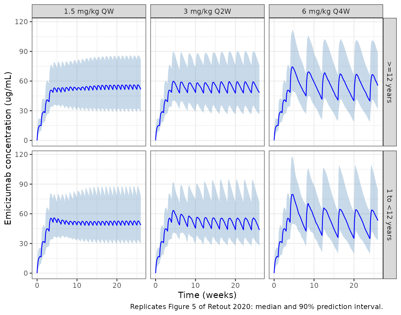
# Negligible age-group difference: median concentration over weeks 5-26,
# pediatric relative to >= 12 years, per regimen. Measured -2.7% to -3.5%:
# weight-based dosing with a CL/F exponent of 0.911 leaves children slightly
# lower, and the F decline above 30 years pulls the adult group partly back.
# The same cohort is drawn on every machine (R's RNG only). With the
# canonical 0.75 exponent instead, children sit 17-18% lower and this
# check fails.
age_diff <- sim_f5 |>
  dplyr::filter(time >= 28) |>
  dplyr::group_by(regimen, age_group) |>
  dplyr::summarise(med = stats::median(Cc), .groups = "drop") |>
  tidyr::pivot_wider(names_from = age_group, values_from = med) |>
  dplyr::mutate(pct = 100 * (`1 to <12 years` / `>=12 years` - 1))
knitr::kable(age_diff, digits = 1, caption = "Median concentration after loading, by age group.")| regimen | 1 to <12 years | >=12 years | pct |
|---|---|---|---|
| 1.5 mg/kg QW | 51.5 | 52.9 | -2.7 |
| 3 mg/kg Q2W | 52.3 | 54.2 | -3.5 |
| 6 mg/kg Q4W | 54.8 | 56.7 | -3.3 |
Assumptions and deviations
-
Correlation between V/F and KA. Table 4 reports
correlations for CL/F-V/F (0.217) and CL/F-KA (-0.341) only. The V/F-KA
covariance is set to 0; the resulting 3 x 3
omegais positive definite. -
CV to variance. Table 4 reports between-person
variability as CV% under an exponential model. It is converted with
omega^2 = log(1 + CV^2). The choice matters only for KA (72.5% CV: 0.422 vs 0.526 with theomega^2 = CV^2approximation). CL/F and V/F change by less than 5%. - Signs of the albumin and age effects. Table 4 prints both coefficients as positive magnitudes. The model follows the Section 3.1 equations, which carry a minus sign. The paper’s own Cav,SS predictions (46.4 and 68.0 ug/mL at 33 and 57 g/L albumin, -31% at 77 years) confirm this; see the closed-form checks above. The Discussion’s phrase “a positive correlation between ALB and CL/F” contradicts both the equation and those predictions, and is not followed.
-
Residual error. Table 4 footnote d specifies a
combined additive-plus-proportional model without the NONMEM coding. It
is encoded as nlmixr2’s
add(addSd) + prop(propSd), with the additive part fixed at 0.025 ug/mL as published. - Age as a baseline covariate. The paper tests covariates at baseline. AGE, WT and ALB are therefore treated as time-fixed per subject.
- Virtual cohort. Individual covariates are not public. Age, weight, albumin and race are drawn from distributions chosen to match the medians and ranges in Tables 2-3; the pediatric weight-for-age curve is an approximation. The paper resampled the observed covariates instead.
- Exposure-bleeding analysis. The annualized-bleeding-rate comparison (Section 2.4, Figure 6) is descriptive and has no model to package.
- Errata. No correction notice for Retout 2020 was found in Crossref or Europe PMC as of 2026-09-27.