Fludarabine (Varela-Gonzalez-Aller 2025)
Source:vignettes/articles/VarelaGonzalezAller_2025_fludarabine.Rmd
VarelaGonzalezAller_2025_fludarabine.RmdModel and source
- Citation: Varela-Gonzalez-Aller J, Sanchez-Salinas MA, Troconiz I, Iacoboni G, Alonso-Martinez C, Carreras-Soler MJ, Carpio C, Farriols-Danes A, Guerra-Gonzalez M, Rivas-Delgado A, Rivera Sanchez L, Feijoo S, Valdivia C, Barba P, Miarons M (2025). Towards Personalized Lymphodepletion: A Population Pharmacokinetic Fludarabine Model in Patients Receiving CAR T-Cell Therapy. Pharmaceutics 17(12):1592. doi:10.3390/pharmaceutics17121592.
- Description: Three-compartment population PK model for intravenous fludarabine (measured as the circulating metabolite F-ara-A) given as lymphodepleting chemotherapy before CD19-directed CAR T-cell therapy in adults with relapsed/refractory large B-cell lymphoma (Varela-Gonzalez-Aller 2025; n = 56 patients, 348 serum samples from 168 infusions). First-order elimination from the central compartment. Clearance is split into an additive non-renal plus renal pair of arms: the non-renal arm depends on which CAR T-cell product the patient was scheduled to receive (4.4 L/h axi-cel vs 3.9 L/h tisa-cel) and the renal arm scales linearly with creatinine clearance normalized to the 96 mL/min cohort median (1.7 L/h at the median). Allometric body-weight scaling is fixed at 0.75 on all three clearance arms and 1 on all three volumes, with a 70 kg reference. Correlated inter-individual variability on CL and V1 (rho = 0.9); log-normal residual error. No exposure-response layer was reported, so only the population PK model is encoded here.
- Article: Pharmaceutics 2025;17(12):1592
- Supplement: Figure S1 (eta distributions)
This is the first population PK model of fludarabine developed exclusively in patients receiving CAR T-cell therapy. Fludarabine is given as the monophosphate prodrug F-ara-AMP but circulates and is assayed as the dephosphorylated metabolite F-ara-A, so every amount in this vignette is an F-ara-A equivalent: the administered F-ara-AMP dose multiplied by the 0.78 molecular-weight ratio the authors used (Methods 2.1.1).
Population
Fifty-six adults with relapsed/refractory large B-cell lymphoma were enrolled prospectively at a single Spanish tertiary centre (Hospital Universitari Vall d’Hebron, Barcelona) between January 2021 and July 2022; 60 were enrolled and 4 excluded for not completing the fludarabine regimen per protocol. Thirty-three (59%) were male and the median age was 59 years (range 23-82). Mean weight was 79.6 kg (SD 12.9; median 82.5, range 52-101) and mean body mass index 25.2 kg/m^2 (SD 3.5; median 25.3, range 18.0-36.2), with obesity documented in two patients. Renal function (Cockcroft-Gault, labelled eGFR in Table 1) averaged 90 mL/min with a range of 39.0-213.9; the cohort median of 96 mL/min is the normalizing constant in the model’s renal clearance arm. Thirty-eight (68%) patients were scheduled for axicabtagene ciloleucel and 18 (32%) for tisagenlecleucel. Histology was diffuse large B-cell lymphoma in 30 (54%), transformed indolent lymphoma in 20 (36%), high-grade B-cell lymphoma in 3 (5%) and other in 3 (5%); 21 (37%) had a prior stem-cell transplant and 11 (20%) had received three or more prior lines. Baseline characteristics are Table 1 of the source.
Lymphodepletion was a 30-minute intravenous fludarabine infusion on days -5, -4 and -3 before cell infusion: 30 mg/m^2 with 500 mg/m^2 cyclophosphamide for axi-cel recipients (cumulative 90 mg/m^2) and 25 mg/m^2 with 250 mg/m^2 cyclophosphamide for tisa-cel recipients (cumulative 75 mg/m^2). Six patients received protocol dose reductions for renal impairment (25% for eGFR 45-60 mL/min, 40% for 30-45 mL/min). Of 400 samples drawn across 168 administrations, 348 entered model development (99 at 1.5 h, 97 at 2 h, 94 at 24 h, 51 taken 30 min before cell infusion, and only 7 at 7 h), a median of 6 per patient. Serum F-ara-A was assayed by UPLC-MS/MS over a 1-1000 ng/mL calibration range (LLOQ 1 ng/mL).
The same information is available programmatically via the model’s
population metadata:
pop <- readModelDb("VarelaGonzalezAller_2025_fludarabine")()$population
str(pop, max.level = 1)
#> List of 14
#>  $ species       : chr "human"
#>  $ n_subjects    : int 56
#>  $ n_studies     : int 1
#>  $ age_range     : chr "23 to 82 years"
#>  $ age_median    : chr "59 years"
#>  $ weight_range  : chr "52 to 101 kg"
#>  $ weight_median : chr "82.5 kg (mean 79.6 +/- 12.9)"
#>  $ sex_female_pct: num 41.1
#>  $ race_ethnicity: NULL
#>  $ disease_state : chr "Relapsed/refractory large B-cell lymphoma (LBCL) after two or more lines of systemic therapy: diffuse large B-c"| __truncated__
#>  $ renal_function: chr "Cockcroft-Gault renal function (labelled eGFR in Table 1) mean 90, range 39.0-213.9 mL/min; cohort median 96 mL"| __truncated__
#>  $ dose_range    : chr "Fludarabine phosphate as a 30-minute intravenous infusion on days -5, -4 and -3 before CAR T-cell infusion, com"| __truncated__
#>  $ regions       : chr "Spain (single centre: Hospital Universitari Vall d'Hebron, Barcelona)."
#>  $ notes         : chr "Prospective, observational, single-centre study conducted January 2021 to July 2022. Sixty patients enrolled, 5"| __truncated__
Source trace
The per-parameter origin is recorded as an in-file comment next to
each ini() entry in
inst/modeldb/specificDrugs/VarelaGonzalezAller_2025_fludarabine.R.
The table below collects them in one place for review. Table 2 of the
source carries the parameter estimates; the covariate model is the
unnumbered equation block printed immediately above Table 2 on page
9.
| Equation / parameter | Value | Source location |
|---|---|---|
CL = [CL_non-renal + CL_renal] * f(WGT) |
n/a | Equation block above Table 2, p. 9; Table 2 CL
Description column |
lcl_nonren (axi-cel non-renal arm) |
4.4 L/h (RSE 1.2%) | Table 2, CL row, theta_CART=1
|
e_tisacel_cl_nonren |
3.9 / 4.4 = 0.8864 | Table 2, CL row, theta_CART=2 = 3.9 (RSE
0.9%) |
lcl_renal (renal arm at CRCL 96) |
1.7 L/h (RSE 1.0%) | Table 2, CL row, theta_CRCL;
CL_renal = theta_CRCL * CRCL/96
|
lvc (V1) |
41.2 L (RSE 9.3%) | Table 2, V1 row, theta_V1
|
lvp (V2, shallow) |
14.5 L (RSE 14.0%) | Table 2, V2 row, theta_V2
|
lvp2 (V3, deep) |
10.8 L (RSE 3.0%) | Table 2, V3 row, theta_V3
|
lq (CLD2) |
4.8 L/h (RSE 5.3%) | Table 2, CLD2 row, theta_CLD2
|
lq2 (CLD3) |
3.6 L/h (RSE 0.1%) | Table 2, CLD3 row, theta_CLD3
|
e_wt_cl_q |
0.75, fixed | Table 2 footnote f(WGT) = (WGT/70)^3/4
|
e_wt_vc_vp |
1.0, fixed | Table 2 footnote g(WGT) = WGT/70
|
etalcl variance |
0.0851 (from 29.8% CV) | Table 2 IIV on CL (%) = 29.8 (RSE 25.1, shrinkage
8.9) |
etalvc variance |
0.1143 (from 34.8% CV) | Table 2 IIV on V1 (%) = 34.8 (RSE 3.6, shrinkage
18.3) |
etalcl-etalvc covariance |
0.0888 (rho = 0.9) | Note printed above Table 2; Results 3.3 block covariance matrix |
expSd |
0.29 (RSE 18.6%) | Table 2 Error [log(ng/mL)] row |
| Three-compartment mammillary ODEs, first-order elimination | n/a | Results 3.3; Discussion paragraph 1 |
| Dose conversion F-ara-AMP -> F-ara-A x 0.78 | n/a | Methods 2.1.1 |
The IIV variances are back-transformed from the reported %CV using
the transform the paper states explicitly in the note above Table 2,
CV(%) = sqrt(exp(omega^2) - 1) * 100; the round-trip is
verified below.
ui  <- rxode2::rxode(readModelDb("VarelaGonzalezAller_2025_fludarabine"))
#> ℹ parameter labels from comments will be replaced by 'label()'
om  <- ui$omega
cv  <- 100 * sqrt(exp(diag(om)) - 1)
rho <- om[1, 2] / sqrt(om[1, 1] * om[2, 2])
tibble::tibble(
  quantity  = c("IIV on CL (%CV)", "IIV on V1 (%CV)", "rho(CL, V1)"),
  published = c(29.8, 34.8, 0.9),
  encoded   = round(c(cv[["etalcl"]], cv[["etalvc"]], rho), 4)
) |>
knitr::kable(caption = "Round-trip of the encoded OMEGA back to the published %CV and correlation.")| quantity | published | encoded |
|---|---|---|
| IIV on CL (%CV) | 29.8 | 29.8037 |
| IIV on V1 (%CV) | 34.8 | 34.7978 |
| rho(CL, V1) | 0.9 | 0.9004 |
Virtual cohort
Original observed data are not publicly available (Data Availability Statement: available on request from the corresponding author). The simulations below use virtual populations whose covariate distributions approximate the published demographics, 200 participants per CAR T-cell-product arm.
Body surface area is needed because dosing is per m^2, but the paper
does not tabulate BSA or height. Both are derived from the two
distributions it does report: height follows from weight and BMI as
sqrt(WT / BMI), and BSA from the Mosteller formula
sqrt(height_cm * WT / 3600). At the reported medians (82.5
kg, 25.3 kg/m^2) this gives 181 cm and 2.03 m^2.
set.seed(20251210)

# Truncated draw helper: sample from `rgen` and resample anything outside
# [lo, hi] rather than clamping, which would pile mass onto the bounds.
rtrunc <- function(n, rgen, lo, hi) {
  x <- rgen(n)
  bad <- which(x < lo | x > hi)
  while (length(bad) > 0L) {
    x[bad] <- rgen(length(bad))
    bad <- which(x < lo | x > hi)
  }
  x
}

# Protocol renal dose reduction (Methods 2.1.1): 25% for eGFR 45-60 mL/min,
# 40% for 30-45 mL/min, none above 60.
dose_reduction <- function(crcl) {
  dplyr::case_when(
    crcl >= 45 & crcl < 60 ~ 0.75,
    crcl >= 30 & crcl < 45 ~ 0.60,
    TRUE                   ~ 1.00
  )
}

make_cohort <- function(n, tisacel, mg_m2, id_offset = 0L) {
  wt  <- rtrunc(n, \(k) rnorm(k, mean = 79.6, sd = 12.9), lo = 52,   hi = 101)
  bmi <- rtrunc(n, \(k) rnorm(k, mean = 25.2, sd = 3.5),  lo = 18.0, hi = 36.2)
  # Median 96 mL/min (Discussion) with a spread covering the Table 1 range.
  crcl <- rtrunc(n, \(k) rlnorm(k, meanlog = log(96), sdlog = 0.40),
                 lo = 39.0, hi = 213.9)
  ht_cm <- 100 * sqrt(wt / bmi)
  bsa   <- sqrt(ht_cm * wt / 3600)
  tibble::tibble(
    id             = id_offset + seq_len(n),
    WT             = wt,
    BMI            = bmi,
    CRCL           = crcl,
    HT             = ht_cm,
    BSA            = bsa,
    CONMED_TISACEL = as.integer(tisacel),
    cohort         = if (tisacel) "tisa-cel (25 mg/m2)" else "axi-cel (30 mg/m2)",
    # F-ara-A equivalent dose in mg: per-m2 F-ara-AMP dose x BSA x protocol
    # renal reduction x the 0.78 molecular-weight ratio (Methods 2.1.1).
    dose_mg        = mg_m2 * bsa * dose_reduction(crcl) * 0.78
  )
}

subjects <- dplyr::bind_rows(
  make_cohort(200, tisacel = FALSE, mg_m2 = 30, id_offset =   0L),
  make_cohort(200, tisacel = TRUE,  mg_m2 = 25, id_offset = 200L)
)

covariate_summary <- subjects |>
  dplyr::summarise(
    dplyr::across(
      c(WT, BMI, CRCL, HT, BSA, dose_mg),
      list(mean = mean, median = stats::median,
           p10 = \(x) stats::quantile(x, 0.10),
           p90 = \(x) stats::quantile(x, 0.90)),
      .names = "{.col}__{.fn}"
    )
  ) |>
  tidyr::pivot_longer(dplyr::everything(),
                      names_to = c("covariate", "statistic"),
                      names_sep = "__") |>
  tidyr::pivot_wider(names_from = statistic, values_from = value)

covariate_summary |>
  dplyr::rename("Covariate" = covariate, "Mean" = mean, "Median" = median,
                "10th pct" = p10, "90th pct" = p90) |>
  knitr::kable(digits = 2,
caption = "Simulated virtual-cohort covariate distributions (n = 400).")| Covariate | Mean | Median | 10th pct | 90th pct |
|---|---|---|---|---|
| WT | 79.38 | 80.04 | 63.81 | 94.88 |
| BMI | 24.96 | 24.99 | 20.41 | 28.93 |
| CRCL | 101.64 | 96.43 | 58.85 | 153.30 |
| HT | 179.10 | 177.94 | 155.37 | 203.14 |
| BSA | 1.99 | 1.99 | 1.68 | 2.30 |
| dose_mg | 41.30 | 41.25 | 32.00 | 50.27 |
The event table is materialized as a plain data frame so the
covariate columns survive into rxSolve(). Observation rows
use cmt = "central" – the ODE state, never the algebraic
observable Cc.
# Rich single-dose grid: dense through distribution, out to 240 h so the
# terminal phase is fully resolved for AUCinf and lambda.z.
obs_times <- sort(unique(c(
  seq(0,   4,  by = 0.05),
  seq(4,   24, by = 0.25),
  seq(24,  96, by = 1),
  seq(96,  240, by = 4)
)))

dose_rows <- subjects |>
  dplyr::mutate(time = 0, amt = dose_mg, evid = 1L, dur = 0.5,
                cmt = "central")

obs_rows <- subjects |>
  tidyr::crossing(time = obs_times) |>
  dplyr::mutate(amt = NA_real_, evid = 0L, dur = NA_real_,
                cmt = "central")

events_single <- dplyr::bind_rows(dose_rows, obs_rows) |>
  dplyr::arrange(id, time, dplyr::desc(evid)) |>
  as.data.frame()

# Guard: IDs must be disjoint across arms and (id, time, evid) unique.
stopifnot(
  dplyr::n_distinct(subjects$id) == nrow(subjects),
  !anyDuplicated(events_single[, c("id", "time", "evid")])
)
nrow(events_single)
#> [1] 108000
Simulation
mod <- readModelDb("VarelaGonzalezAller_2025_fludarabine")

sim_single <- rxode2::rxSolve(
  mod,
  events = events_single,
  keep   = c("cohort", "WT", "CRCL", "BSA", "dose_mg", "CONMED_TISACEL")
) |>
  as.data.frame()
#> ℹ parameter labels from comments will be replaced by 'label()'

stopifnot(nrow(sim_single) > 0, all(sim_single$Cc >= 0, na.rm = TRUE))
Structural gate: AUC equals dose divided by clearance
For a linear model with intravenous input the extrapolated AUC must
equal dose / CL exactly. Checking this on a typical-value
solve (random effects zeroed) validates the whole clearance block – both
arms, the additive combination, the allometric exponent and the
mg-to-ng/mL scale factor – against closed-form arithmetic rather than
against a figure.
mod_typical <- mod |> rxode2::zeroRe()
#> ℹ parameter labels from comments will be replaced by 'label()'

# Typical patient: 70 kg (the allometric reference), CRCL 96 mL/min (the
# cohort median), i.e. exactly the patient the Discussion quotes.
typ_bsa  <- sqrt(100 * sqrt(70 / 25.3) * 70 / 3600)
typ_dose <- c("axi-cel (30 mg/m2)" = 30, "tisa-cel (25 mg/m2)" = 25) * typ_bsa * 0.78

typ_subjects <- tibble::tibble(
  id             = 1:2,
  WT             = 70,
  CRCL           = 96,
  CONMED_TISACEL = c(0L, 1L),
  cohort         = names(typ_dose),
  dose_mg        = as.numeric(typ_dose)
)

typ_events <- dplyr::bind_rows(
  typ_subjects |> dplyr::mutate(time = 0, amt = dose_mg, evid = 1L,
                                dur = 0.5, cmt = "central"),
  typ_subjects |> tidyr::crossing(time = obs_times) |>
    dplyr::mutate(amt = NA_real_, evid = 0L, dur = NA_real_, cmt = "central")
) |>
  dplyr::arrange(id, time, dplyr::desc(evid)) |>
  as.data.frame()

sim_typ <- rxode2::rxSolve(
  mod_typical, events = typ_events,
  keep = c("cohort", "dose_mg"), atol = 1e-10, rtol = 1e-10
) |>
  as.data.frame()
#> ℹ omega/sigma items treated as zero: 'etalcl', 'etalvc'
#> Warning: multi-subject simulation without without 'omega'

mass_balance <- sim_typ |>
  dplyr::group_by(cohort) |>
  dplyr::summarise(
    CL_model  = dplyr::first(cl),
    dose_mg   = dplyr::first(dose_mg),
    # Trapezoidal AUC over the simulated window, ng*h/mL.
    AUC_num   = sum(diff(time) * (head(Cc, -1) + tail(Cc, -1)) / 2),
    .groups   = "drop"
  ) |>
  # dose (mg) -> ng: x 1e6; AUC in ng*h/mL = ng*h/mL, so dose_ng / AUC gives mL/h
  # -> divide by 1000 for L/h. Net: dose_mg * 1000 / AUC = CL in L/h.
  dplyr::mutate(
    AUC_closed_form = dose_mg * 1000 / CL_model,
    ratio           = AUC_num / AUC_closed_form
  )

mass_balance |>
  dplyr::rename("Arm" = cohort, "CL (L/h)" = CL_model, "Dose (mg)" = dose_mg,
                "AUC numeric (ng*h/mL)" = AUC_num,
                "Dose/CL (ng*h/mL)" = AUC_closed_form, "Ratio" = ratio) |>
  knitr::kable(digits = c(0, 4, 2, 1, 1, 6),
caption = "Mass-balance gate: numeric AUC vs. the closed-form dose/CL.")| Arm | CL (L/h) | Dose (mg) | AUC numeric (ng*h/mL) | Dose/CL (ng*h/mL) | Ratio |
|---|---|---|---|---|---|
| axi-cel (30 mg/m2) | 6.1 | 42.08 | 6899.7 | 6898.9 | 1.000114 |
| tisa-cel (25 mg/m2) | 5.6 | 35.07 | 6263.1 | 6262.4 | 1.000111 |
# The two arms must reproduce the Discussion's typical clearances exactly, and
# the numeric AUC must agree with dose/CL to within integration error.
stopifnot(
  isTRUE(all.equal(mass_balance$CL_model[mass_balance$cohort == "axi-cel (30 mg/m2)"],
                   6.1, tolerance = 1e-6)),
  isTRUE(all.equal(mass_balance$CL_model[mass_balance$cohort == "tisa-cel (25 mg/m2)"],
                   5.6, tolerance = 1e-6)),
  all(abs(mass_balance$ratio - 1) < 1e-3)
)
Structural gate: analytic terminal half-life
The three-compartment micro-constants imply a terminal disposition rate that can be obtained analytically as the smallest root of the characteristic cubic. The log-linear slope fitted to the far tail of the simulation must recover it.
mc <- sim_typ |> dplyr::filter(cohort == "axi-cel (30 mg/m2)") |> dplyr::slice(1)
k10 <- mc$kel; k12 <- mc$k12; k21 <- mc$k21; k13 <- mc$k13; k31 <- mc$k31

# Characteristic polynomial of the 3-compartment mammillary system, written
# for the positive decay rates u (concentrations decay as exp(-u t)):
#   u^3 - a2 u^2 + a1 u - a0 = 0
# so the coefficient vector passed to polyroot() alternates in sign.
a2 <- k10 + k12 + k21 + k13 + k31
a1 <- k10 * k21 + k10 * k31 + k12 * k31 + k13 * k21 + k21 * k31
a0 <- k10 * k21 * k31
roots  <- sort(Re(polyroot(c(-a0, a1, -a2, 1))))
gamma  <- roots[1]                       # slowest (terminal) rate
t_half <- log(2) / gamma

# Keep Cc >= 1e-6 of Cmax (below that the ODE tail is solver noise). The floor
# ends the window near 160 h, so it opens at 96 h, long after the beta phase.
tail_fit <- sim_typ |>
  dplyr::filter(cohort == "axi-cel (30 mg/m2)") |>
  dplyr::filter(time >= 96, time <= 240, Cc >= 1e-6 * max(Cc))
t_half_fitted <- -log(2) / stats::coef(stats::lm(log(Cc) ~ time, tail_fit))[[2]]

tibble::tibble(
  quantity = c("alpha (1/h)", "beta (1/h)", "gamma (1/h)",
               "terminal t-half, analytic (h)", "terminal t-half, fitted from 96 h (h)"),
  value    = c(roots[3], roots[2], gamma, t_half, t_half_fitted)
) |>
  dplyr::rename("Quantity" = quantity, "Value" = value) |>
knitr::kable(digits = 4, caption = "Analytic vs. fitted terminal disposition.")| Quantity | Value |
|---|---|
| alpha (1/h) | 0.6024 |
| beta (1/h) | 0.3323 |
| gamma (1/h) | 0.0816 |
| terminal t-half, analytic (h) | 8.4934 |
| terminal t-half, fitted from 96 h (h) | 8.4934 |
Replicate published figures
# Replicates Figure 1 of Varela-Gonzalez-Aller 2025: serum fludarabine
# (F-ara-A) concentration-time profiles following the first intravenous
# infusion. The published panel shows raw observations over roughly the first
# 24 h; the ribbon here is the simulated 2.5th-97.5th percentile band with the
# assay calibration range marked.
sim_single |>
  dplyr::filter(time > 0, time <= 24) |>
  dplyr::group_by(time) |>
  dplyr::summarise(
    Q025 = stats::quantile(Cc, 0.025),
    Q50  = stats::quantile(Cc, 0.500),
    Q975 = stats::quantile(Cc, 0.975),
    .groups = "drop"
  ) |>
  ggplot(aes(time, Q50)) +
  geom_ribbon(aes(ymin = Q025, ymax = Q975), alpha = 0.25) +
  geom_line(linewidth = 0.8) +
  geom_hline(yintercept = c(1, 1000), linetype = "dotted") +
  scale_y_log10() +
  labs(
    x = "Time after the start of the first infusion (h)",
    y = "Serum F-ara-A (ng/mL)",
    title = "Figure 1 - profiles after the first intravenous injection",
    caption = paste(
      "Replicates Figure 1 of Varela-Gonzalez-Aller 2025. Line = simulated",
      "median, band = 2.5th-97.5th percentiles (n = 400).",
      "Dotted lines mark the 1-1000 ng/mL assay calibration range."
    )
  )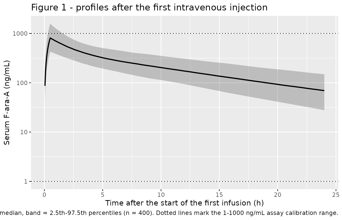
Figure 4 of the source shows typical profiles across the 10th, 50th and 90th percentiles of weight and of eGFR, and across the two CAR T-cell products, with the dose held constant across every scenario (“The dose administered in each simulation remained constant across all scenarios and patients”). The panel layout follows the published caption: the median weight is used in the left and right panels, the median eGFR in the left and middle panels, and the axi-cel construct in the middle and right panels. Percentiles are taken from the simulated cohort because the paper does not tabulate them.
pct <- function(covariate, p) {
  v <- covariate_summary[covariate_summary$covariate == covariate, ]
  as.numeric(v[[p]])
}
wt_p   <- c(`10th` = pct("WT", "p10"),   `50th` = pct("WT", "median"),   `90th` = pct("WT", "p90"))
crcl_p <- c(`10th` = pct("CRCL", "p10"), `50th` = pct("CRCL", "median"), `90th` = pct("CRCL", "p90"))

# Constant dose across every scenario, per the published caption.
fixed_dose <- 30 * typ_bsa * 0.78

# Three-day lymphodepletion course: 30-min infusions at 0, 24 and 48 h.
scen_times <- sort(unique(c(seq(0, 120, by = 0.25))))

scenarios <- dplyr::bind_rows(
  tibble::tibble(panel = "eGFR (median weight, axi-cel)",
                 level = names(crcl_p), WT = wt_p[["50th"]],
                 CRCL = as.numeric(crcl_p), CONMED_TISACEL = 0L),
  tibble::tibble(panel = "CAR-T construct (median weight and eGFR)",
                 level = c("axi-cel", "tisa-cel"), WT = wt_p[["50th"]],
                 CRCL = crcl_p[["50th"]], CONMED_TISACEL = c(0L, 1L)),
  tibble::tibble(panel = "Weight (median eGFR, axi-cel)",
                 level = names(wt_p), WT = as.numeric(wt_p),
                 CRCL = crcl_p[["50th"]], CONMED_TISACEL = 0L)
) |>
  dplyr::mutate(id = dplyr::row_number())

scen_events <- dplyr::bind_rows(
  scenarios |> tidyr::crossing(time = c(0, 24, 48)) |>
    dplyr::mutate(amt = fixed_dose, evid = 1L, dur = 0.5, cmt = "central"),
  scenarios |> tidyr::crossing(time = scen_times) |>
    dplyr::mutate(amt = NA_real_, evid = 0L, dur = NA_real_, cmt = "central")
) |>
  dplyr::arrange(id, time, dplyr::desc(evid)) |>
  as.data.frame()

sim_scen <- rxode2::rxSolve(
  mod_typical, events = scen_events, keep = c("panel", "level")
) |>
  as.data.frame()
#> ℹ omega/sigma items treated as zero: 'etalcl', 'etalvc'
#> Warning: multi-subject simulation without without 'omega'

sim_scen |>
  dplyr::filter(time > 0) |>
  ggplot(aes(time, Cc, colour = level)) +
  geom_line(linewidth = 0.7) +
  facet_wrap(~panel) +
  scale_y_log10() +
  labs(
    x = "Time after the first infusion (h)", y = "Serum F-ara-A (ng/mL)",
    colour = "Level",
    title = "Figure 4 - impact of the selected covariates on typical profiles",
    caption = paste(
      "Replicates Figure 4 of Varela-Gonzalez-Aller 2025. Typical-value",
      "profiles (random effects zeroed) over the three-day lymphodepletion",
      "course, dose held constant across all scenarios."
    )
  ) +
  theme(legend.position = "bottom")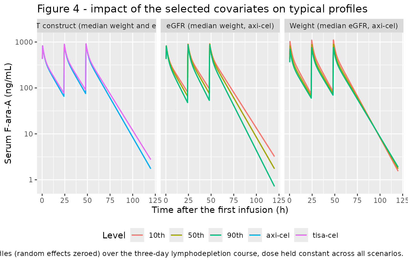
The source makes one quantitative claim about this figure: eGFR produces “a five-fold difference between the 10th and 90th percentiles at final simulated time points”. That is checkable.
egfr_fold <- sim_scen |>
  dplyr::filter(panel == "eGFR (median weight, axi-cel)",
                time == max(time)) |>
  dplyr::select(level, Cc) |>
  tidyr::pivot_wider(names_from = level, values_from = Cc) |>
  dplyr::mutate(fold_10th_over_90th = `10th` / `90th`)

egfr_fold |>
  dplyr::rename("Cc at 10th pct eGFR" = `10th`, "Cc at 50th pct" = `50th`,
                "Cc at 90th pct eGFR" = `90th`,
                "Fold difference (10th/90th)" = fold_10th_over_90th) |>
  knitr::kable(digits = 3,
               caption = paste(
                 "Terminal-timepoint fold difference across the eGFR",
                 "percentiles; the source reports approximately five-fold."
))| Cc at 10th pct eGFR | Cc at 50th pct | Cc at 90th pct eGFR | Fold difference (10th/90th) |
|---|---|---|---|
| 3.209 | 1.738 | 0.718 | 4.466 |
The simulated fold difference is of the order the paper describes, and the direction is the one it reports – patients with impaired eGFR show progressive accumulation and delayed elimination. The exact multiple depends on the eGFR percentiles, which the paper does not tabulate; see Assumptions below.
PKNCA validation
NCA is run on the single-dose cohort simulation. The time-zero row
that anchors AUC is always kept (a time > 0 or
Cc > 0 filter would drop it); points past each subject’s
peak that fall below 1e-6 of it, where the solved profile is numerical
noise, are dropped before the half-life fit.
sim_nca <- sim_single |>
  dplyr::filter(!is.na(Cc)) |>
  # Per subject, keep Cc >= 1e-6 of Cmax after the peak: below that the ODE tail is solver noise.
  dplyr::group_by(id) |>
  dplyr::filter(time <= time[which.max(Cc)] | Cc >= 1e-6 * max(Cc)) |>
  dplyr::ungroup() |>
  dplyr::select(id, time, Cc, cohort)

# Guarantee a time = 0 row per (id, cohort). For intravenous input the
# pre-dose concentration is 0.
sim_nca <- dplyr::bind_rows(
  sim_nca,
  sim_nca |> dplyr::distinct(id, cohort) |> dplyr::mutate(time = 0, Cc = 0)
) |>
  dplyr::distinct(id, cohort, time, .keep_all = TRUE) |>
  dplyr::arrange(id, cohort, time)

conc_obj <- PKNCA::PKNCAconc(sim_nca, Cc ~ time | cohort + id)

dose_df <- events_single |>
  dplyr::filter(evid == 1) |>
  dplyr::select(id, time, amt, cohort)

dose_obj <- PKNCA::PKNCAdose(dose_df, amt ~ time | cohort + id)

intervals <- data.frame(
  start      = 0,
  end        = Inf,
  cmax       = TRUE,
  tmax       = TRUE,
  aucinf.obs = TRUE,
  half.life  = TRUE,
  cl.obs     = TRUE,
  vss.iv.obs = TRUE,
  mrt.iv.obs = TRUE
)

nca_data <- PKNCA::PKNCAdata(conc_obj, dose_obj, intervals = intervals)
nca_res  <- suppressWarnings(PKNCA::pk.nca(nca_data))

nca_summary <- as.data.frame(nca_res) |>
  dplyr::filter(!is.na(PPORRES)) |>
  dplyr::group_by(cohort, PPTESTCD) |>
  dplyr::summarise(median = stats::median(PPORRES),
                   p05 = stats::quantile(PPORRES, 0.05),
                   p95 = stats::quantile(PPORRES, 0.95),
                   .groups = "drop")

nca_summary |>
  dplyr::mutate(PPTESTCD = nlmixr2lib::ncaParamLabel(PPTESTCD)) |>
  dplyr::rename("Arm" = cohort, "NCA parameter" = PPTESTCD,
                "Median" = median, "5th pct" = p05, "95th pct" = p95) |>
  knitr::kable(digits = 5,
               caption = paste(
                 "Cohort NCA of the simulated first dose. CL and Vss are on",
                 "the raw dose/AUC scale here -- see the unit note below."
               ))
#> Warning: There was 1 warning in `dplyr::mutate()`.
#> ℹ In argument: `PPTESTCD = nlmixr2lib::ncaParamLabel(PPTESTCD)`.
#> Caused by warning:
#> ! ncaParamLabel(): unknown PKNCA code(s) returned as-is: 'adj.r.squared', 'clast.pred', 'lambda.z.time.first', 'lambda.z.time.last', 'r.squared', 'span.ratio'| Arm | NCA parameter | Median | 5th pct | 95th pct |
|---|---|---|---|---|
| axi-cel (30 mg/m2) | adj.r.squared | 0.99990 | 0.99990 | 0.99991 |
| axi-cel (30 mg/m2) | AUC0-∞ (obs) | 6674.46183 | 4058.01288 | 11120.87600 |
| axi-cel (30 mg/m2) | AUMC0-∞ (obs) | 79080.06867 | 37450.44273 | 163991.11099 |
| axi-cel (30 mg/m2) | CL/F | 0.00656 | 0.00393 | 0.01177 |
| axi-cel (30 mg/m2) | Clast | 0.00107 | 0.00055 | 0.00199 |
| axi-cel (30 mg/m2) | clast.pred | 0.00104 | 0.00054 | 0.00195 |
| axi-cel (30 mg/m2) | Cmax | 877.57610 | 482.49182 | 1522.06962 |
| axi-cel (30 mg/m2) | t½ | 8.84065 | 6.86783 | 11.92547 |
| axi-cel (30 mg/m2) | λz | 0.07840 | 0.05812 | 0.10093 |
| axi-cel (30 mg/m2) | λz n points | 176.50000 | 163.00000 | 192.10000 |
| axi-cel (30 mg/m2) | lambda.z.time.first | 3.75000 | 3.50000 | 3.95000 |
| axi-cel (30 mg/m2) | lambda.z.time.last | 168.00000 | 128.00000 | 224.00000 |
| axi-cel (30 mg/m2) | MRT (IV) | 11.70377 | 8.82807 | 15.91567 |
| axi-cel (30 mg/m2) | r.squared | 0.99991 | 0.99990 | 0.99991 |
| axi-cel (30 mg/m2) | span.ratio | 18.40592 | 17.94922 | 18.87117 |
| axi-cel (30 mg/m2) | Tlast | 168.00000 | 128.00000 | 224.00000 |
| axi-cel (30 mg/m2) | Tmax | 0.50000 | 0.50000 | 0.50000 |
| axi-cel (30 mg/m2) | Vss (IV) | 0.07726 | 0.05077 | 0.12694 |
| tisa-cel (25 mg/m2) | adj.r.squared | 0.99991 | 0.99990 | 0.99991 |
| tisa-cel (25 mg/m2) | AUC0-∞ (obs) | 5996.86149 | 3797.83091 | 10338.47620 |
| tisa-cel (25 mg/m2) | AUMC0-∞ (obs) | 75655.80696 | 35753.31597 | 159555.00251 |
| tisa-cel (25 mg/m2) | CL/F | 0.00615 | 0.00349 | 0.01028 |
| tisa-cel (25 mg/m2) | Clast | 0.00085 | 0.00052 | 0.00156 |
| tisa-cel (25 mg/m2) | clast.pred | 0.00083 | 0.00051 | 0.00153 |
| tisa-cel (25 mg/m2) | Cmax | 720.98806 | 458.83681 | 1266.45037 |
| tisa-cel (25 mg/m2) | t½ | 9.40089 | 7.09183 | 12.12498 |
| tisa-cel (25 mg/m2) | λz | 0.07373 | 0.05717 | 0.09774 |
| tisa-cel (25 mg/m2) | λz n points | 179.00000 | 166.00000 | 196.00000 |
| tisa-cel (25 mg/m2) | lambda.z.time.first | 3.70000 | 3.45000 | 3.90000 |
| tisa-cel (25 mg/m2) | lambda.z.time.last | 180.00000 | 135.80000 | 228.00000 |
| tisa-cel (25 mg/m2) | MRT (IV) | 12.52621 | 9.26405 | 16.29298 |
| tisa-cel (25 mg/m2) | r.squared | 0.99991 | 0.99990 | 0.99991 |
| tisa-cel (25 mg/m2) | span.ratio | 18.50030 | 17.95311 | 18.85652 |
| tisa-cel (25 mg/m2) | Tlast | 180.00000 | 135.80000 | 228.00000 |
| tisa-cel (25 mg/m2) | Tmax | 0.50000 | 0.50000 | 0.50000 |
| tisa-cel (25 mg/m2) | Vss (IV) | 0.07789 | 0.05060 | 0.11236 |
Unit note. Doses are in mg while concentrations are
in ng/mL (= ug/L), so PKNCA’s dose / AUC is evaluated
numerically without unit reconciliation. One unit of that ratio is
1 mg / (1 ng*h/mL) = 10^6 ng / (1 ng*h/mL) = 10^6 mL/h = 1000 L/h,
so the raw cl.obs and vss.iv.obs values
must be multiplied by 1000 to obtain L/h and L, the
units the paper reports. cmax, tmax,
aucinf.obs, half.life and
mrt.iv.obs carry no dose term and are unaffected.
Comparison against published values
The source reports no NCA table, so the reference column is built
from the typical-value quantities it does publish: the Discussion’s
clearances for “a typical 70 kg patient with a median eGFR value (96
mL/min)” – 6.1 L/h for axi-cel and 5.6 L/h for tisa-cel – and the Table
2 steady-state volume
V1 + V2 + V3 = 41.2 + 14.5 + 10.8 = 66.5 L. Because those
are typical values at a specified weight and renal function, the
comparison uses the typical-value simulation rather than the cohort
median, whose covariate distribution differs from 70 kg / 96 mL/min by
construction.
typ_nca_in <- sim_typ |>
  dplyr::filter(!is.na(Cc)) |>
  # Per subject, keep Cc >= 1e-6 of Cmax after the peak: below that the ODE tail is solver noise.
  dplyr::group_by(id) |>
  dplyr::filter(time <= time[which.max(Cc)] | Cc >= 1e-6 * max(Cc)) |>
  dplyr::ungroup() |>
  dplyr::select(id, time, Cc, cohort)

typ_nca_in <- dplyr::bind_rows(
  typ_nca_in,
  typ_nca_in |> dplyr::distinct(id, cohort) |> dplyr::mutate(time = 0, Cc = 0)
) |>
  dplyr::distinct(id, cohort, time, .keep_all = TRUE) |>
  dplyr::arrange(id, cohort, time)

typ_dose_df <- typ_events |>
  dplyr::filter(evid == 1) |>
  dplyr::select(id, time, amt, cohort)

typ_res <- suppressWarnings(PKNCA::pk.nca(PKNCA::PKNCAdata(
  PKNCA::PKNCAconc(typ_nca_in, Cc ~ time | cohort + id),
  PKNCA::PKNCAdose(typ_dose_df, amt ~ time | cohort + id),
  intervals = intervals
)))

# Rescale the dose-normalized parameters onto L/h and L (see the unit note).
typ_long <- as.data.frame(typ_res) |>
  dplyr::filter(!is.na(PPORRES)) |>
  dplyr::mutate(PPORRES = dplyr::if_else(
    PPTESTCD %in% c("cl.obs", "vss.iv.obs"), PPORRES * 1000, PPORRES
  )) |>
  dplyr::select(cohort, PPTESTCD, PPORRES)

published <- tibble::tribble(
  ~cohort,                ~cl.obs, ~vss.iv.obs,
  "axi-cel (30 mg/m2)",   6.1,     66.5,
  "tisa-cel (25 mg/m2)",  5.6,     66.5
)

cmp <- nlmixr2lib::ncaComparisonTable(
  simulated     = typ_long,
  reference     = published,
  by            = "cohort",
  units         = c(cl.obs = "L/h", vss.iv.obs = "L"),
  tolerance_pct = 20
)

knitr::kable(
  cmp,
  caption = paste(
    "Simulated typical-value NCA vs. the published typical values",
    "(Discussion clearances; Table 2 V1 + V2 + V3).",
    "* differs from reference by >20%."
  )
)| NCA parameter | cohort | Reference | Simulated | % diff |
|---|---|---|---|---|
| CL/F (L/h) | axi-cel (30 mg/m2) | 6.1 | 6.1 | -0.0% |
| CL/F (L/h) | tisa-cel (25 mg/m2) | 5.6 | 5.6 | -0.0% |
| Vss (IV) (L) | axi-cel (30 mg/m2) | 66.5 | 68 | +2.3% |
| Vss (IV) (L) | tisa-cel (25 mg/m2) | 66.5 | 67.9 | +2.1% |
# Make this comparison an actual gate rather than a rendered table: assert the
# achieved agreement, tightened to what the simulation delivers. CL is an exact
# algebraic identity (dose/AUCinf), so it is held to 0.1%. Vss is looser because
# PKNCA derives it as CL x MRT from a numerically integrated AUMC, whose long
# tail is trapezoid-sensitive; 5% is comfortably tighter than the 20% flag.
cl_sim  <- typ_long$PPORRES[typ_long$PPTESTCD == "cl.obs"]
cl_ref  <- published$cl.obs[match(
  typ_long$cohort[typ_long$PPTESTCD == "cl.obs"], published$cohort)]
vss_sim <- typ_long$PPORRES[typ_long$PPTESTCD == "vss.iv.obs"]
stopifnot(
  length(cl_sim) == 2L, length(vss_sim) == 2L,
  all(abs(cl_sim / cl_ref - 1) < 0.001),
  all(abs(vss_sim / 66.5 - 1) < 0.05)
)
Both clearances agree with the published typical values to within
numerical integration error, which is the expected result:
cl.obs is dose / AUCinf, and the mass-balance
gate above already showed AUCinf = dose / CL holds exactly,
so this row is an independent PKNCA-side confirmation of the same
identity. Vss recovers the sum of the three published
volumes to about 2% – PKNCA derives it as CL x MRT from a
numerically integrated AUMC, whose long tail is more trapezoid-sensitive
than the AUC, so exact agreement is not expected. That it lands on 66.5
L at all confirms V2 and V3 are encoded as
true compartment volumes on the g(WGT) scale rather than as
weight-normalized quantities. No row is starred.
For completeness, the descriptive cohort NCA in the previous section brackets these typical values, as it must once the cohort’s weight and renal-function spread is introduced.
nca_summary |>
  dplyr::filter(PPTESTCD == "cl.obs") |>
  dplyr::mutate(dplyr::across(c(median, p05, p95), \(x) x * 1000)) |>
  dplyr::left_join(published |> dplyr::select(cohort, published = cl.obs),
                   by = "cohort") |>
  dplyr::rename("Arm" = cohort, "Cohort median CL (L/h)" = median,
                "5th pct" = p05, "95th pct" = p95,
                "Published typical (L/h)" = published) |>
  dplyr::select(-PPTESTCD) |>
  knitr::kable(digits = 3,
               caption = paste(
                 "Cohort clearance distribution vs. the published typical",
                 "value at 70 kg / 96 mL/min."
))| Arm | Cohort median CL (L/h) | 5th pct | 95th pct | Published typical (L/h) |
|---|---|---|---|---|
| axi-cel (30 mg/m2) | 6.565 | 3.933 | 11.771 | 6.1 |
| tisa-cel (25 mg/m2) | 6.148 | 3.486 | 10.281 | 5.6 |
Assumptions and deviations
-
Allometric reference is 70 kg, not the cohort
median. Methods 2.3.2 says continuous covariates were
“normalized by the median value of the study population”, but the
definitions printed with Table 2 are
f(WGT) = (WGT/70)^3/4andg(WGT) = WGT/70– 70 kg, whereas the cohort median weight is 82.5 kg. The printed equation governs, per the standing policy of trusting the equation over the prose. The Discussion independently confirms it:(4.4 + 1.7) x 1 = 6.1L/h and(3.9 + 1.7) x 1 = 5.6L/h reproduce its quoted clearances exactly for “a typical 70 kg patient”, which is only true whenf(70) = 1. -
theta_CRCLis lost in text extraction but present in the PDF. The value 1.7 L/h (RSE 1.0%) is read from the Table 2CLrow of the source PDF. The mass-balance gate above re-derives it independently from the Discussion’s typical clearances, so it is not taken on trust from a single reading. -
Renal function is recorded as the canonical raw-mL/min
CRCLcolumn. The paper labels it “eGFR” with units mL/min/1.73 m^2 in Table 1, but Methods 2.1.2 states it was computed with the Cockcroft-Gault formula, which returns a non-BSA-normalized mL/min value, and both Table 2 and the Discussion quote it in plain mL/min. Nothing in the model changes either way – it is the same column with the same 96 mL/min reference – but the units field records the Cockcroft-Gault reading. - Table 1 reports mean eGFR 90 mL/min while the Discussion reports median 96. These are mutually consistent only under a left-skewed distribution, which is hard to reconcile with the reported 39.0-213.9 range. The virtual cohort is calibrated to the median of 96 because that is the value the model’s renal arm normalizes by; the achieved cohort mean is reported in the covariate-summary table above and is higher than 90.
- eGFR and weight percentiles are simulated, not published. Figure 4 uses the 10th, 50th and 90th percentiles of each covariate, but the paper tabulates only means, medians and ranges. The percentiles here come from the virtual cohort, so the reproduced fold differences are of the published order rather than exact matches.
-
Height and BSA are derived, not reported. Dosing is
per m^2 but the paper tabulates neither height nor BSA. Height is
recovered from the reported weight and BMI distributions as
sqrt(WT / BMI)and BSA from the Mosteller formula. Any other BSA formula would shift absolute concentrations slightly but cannot affect the clearance and volume comparisons, which are dose-normalized. -
Doses are F-ara-A equivalents. The model describes
the circulating metabolite F-ara-A, and the authors scaled every
administered F-ara-AMP dose by 0.78 before fitting (Methods 2.1.1). The
factor is applied in the vignette event tables, not inside
model(), because it is a property of the dose record rather than of the model. Passing an unconverted F-ara-AMP amount would overstate exposure by 1/0.78 = 1.28-fold. -
The CAR T-cell product covariate is a cohort marker, not an
interaction.
CONMED_TISACELis registered in theCONMED_<INN>family, but the cell product is infused on day 0 whereas fludarabine is given on days -5 to -3 and the last PK sample is drawn 30 min before the infusion – the product has not been administered during any modelled observation. The authors state that the effect “is unlikely to be clinically meaningful and may instead reflect unmeasured covariates or other patient-specific factors”. Treat it as a proxy for population differences between the two product cohorts. - Time-varying covariates are held constant. The paper measured renal function at two occasions (pre-lymphodepletion and before the third dose) and treated it as time-varying; the simulations here assign one value per subject for the whole course.
- Inter-occasion variability was explored but not retained. Methods 2.3.1 states IOV was investigated; Table 2 reports no IOV term, so none is encoded.
- No IIV on CLD2, CLD3, V2 or V3, by design. Results 3.3 states these were excluded for lack of statistical or clinical evidence and insufficient precision, so the encoded model has random effects only on CL and V1.
-
Residual error is log-normal, not proportional.
Table 2 reports
Error [log(ng/mL)] = 0.29on log-transformed data, encoded asCc ~ lnorm(expSd). Because the error is additive on the log scale it is invariant to the mg/L-to-ng/mL rescaling ofCc. -
The 7 h sampling window is sparse in the source.
Only 7 of 348 samples were drawn at 7 h, and the authors flag reduced
precision on
V3andCLD3(which govern the beta/gamma transition) as a limitation. The simulated terminal phase inherits that uncertainty despite the tight reported RSEs. - No exposure-response layer. The paper explicitly does not analyse AUC against neurotoxicity, cytokine release syndrome or CAR T-cell expansion, so only the population PK model is packaged. ```