Dabigatran sheep (Eaton 2025) • nlmixr2lib

Model and source

#> ℹ parameter labels from comments will be replaced by 'label()'

Citation: Eaton MP, Nadtochiy SM, Stefanos T, Anderson BJ. Dabigatran pharmacokinetic-pharmacodynamic in sheep: Informing dose for anticoagulation during cardiopulmonary bypass. Perfusion. 2025;40(1):183-191. doi:10.1177/02676591231226291
Description: Preclinical (sheep). Integrated two-compartment IV pharmacokinetic plus effect-compartment sigmoid Emax pharmacodynamic model for dabigatran and its reversal agent idarucizumab in anaesthetised sheep, describing thromboelastographic reaction time (R-time). Parameters are allometrically standardised to a 70 kg body weight for cross-species comparison (Eaton 2025 Tables 2-3 and the supplementary NM-TRAN control stream).
Article: https://doi.org/10.1177/02676591231226291
Supplementary NM-TRAN control stream and Supplementary Figures S1-S2 are distributed with the article as supplementary material (open access, PMC11715065).

Eaton and colleagues gave five anaesthetised sheep dabigatran 4 mg/kg intravenously, reversed it with idarucizumab 15 mg/kg at 120 min, and fitted an integrated pharmacokinetic-pharmacodynamic model to plasma dabigatran concentrations and thromboelastographic reaction time (R-time). The purpose of the analysis was to apply the target-concentration strategy: identify the dabigatran concentration associated with an acceptable anticoagulant effect, and back out a loading dose plus maintenance infusion that reaches it for sheep undergoing cardiopulmonary bypass.

The packaged model reproduces the published structure exactly: two-compartment dabigatran disposition, an effect compartment linked to the central compartment by ke0, a sigmoid Emax function relating effect-site concentration to R-time, and a K-PD compartment carrying a unit idarucizumab dose whose amount reduces R-time linearly.

Population

Five female sheep, all 6 months old, weighing 28.7, 33.9, 33.8, 33.9 and 41.8 kg (Eaton 2025 Table 1). All animals were studied under general anaesthesia (ketamine plus midazolam induction, isoflurane maintenance). Each received dabigatran 4 mg/kg intravenously over 1 min at time 0, and idarucizumab 15 mg/kg over 30 s at 120 min. Plasma dabigatran and R-time were sampled at baseline and 5, 15, 30, 60, 90 and 120 min after dabigatran, then 5, 15, 30, 60, 120, 240 and 480 min and 24 h after idarucizumab. Markers of hepatic and renal injury (ALT, AST, creatinine) were unchanged at 24 h.

Parameters in Table 2 and Table 3 are reported standardised to a 70 kg body weight using allometric scaling, so that the sheep estimates can be compared against published adult-human values. That 70 kg standard is a reporting convention: no sheep in the study weighed anything close to it.

The same information is available programmatically via the model’s population metadata (readModelDb("Eaton_2025_dabigatran_sheep")()$population).

Source trace

The per-parameter origin is recorded as an in-file comment next to each ini() entry in inst/modeldb/specificDrugs/Eaton_2025_dabigatran_sheep.R. The table below collects them in one place for review.

Equation / parameter	Value	Source location
`lcl`	CL 0.0453 L/min/70 kg	Eaton 2025 Table 2
`lvc`	V1 2.94 L/70 kg	Eaton 2025 Table 2
`lq`	Q 0.268 L/min/70 kg	Eaton 2025 Table 2
`lvp`	V2 9.51 L/70 kg	Eaton 2025 Table 2
`e_wt_cl_q`	0.75	Eaton 2025 Methods Eq. 1; supplement `FSZCL = (WT/70)**0.75`
`e_wt_vc_vp`	1	Eaton 2025 Methods Eq. 1; supplement `FSZV = WT/70`
`le0`	E0 0.681 min	Eaton 2025 Table 3
`lemax`	Emax 180 min FIX	Eaton 2025 Table 3; supplement `$THETA (100,180.,300) FIX`
`lec50`	Ce50 64.2 mg/L	Eaton 2025 Table 3
`lhill`	N 1 FIX	Eaton 2025 Table 3
`lke0`	T1/2keo 1.04 min, ke0 = ln(2)/1.04	Eaton 2025 Table 3; supplement `KEQ = LN2/TEQ`
`e_wt_ke0`	-0.25	supplement `FSZT = (WT/70)**0.25` applied to T1/2keo
`lkel_ida`	KIDA 0.0218 1/min	Eaton 2025 Table 3
`ldur_ida`	DURIDA 0.0751 min	Eaton 2025 Table 3; supplement `D4 = DURIDA`
`lslope_ida`	SLOPEIDA 8.24 min per unit dose	Eaton 2025 Table 3
`etalcl`, `etalvc`, `etalq`, `etalvp`	%BSV 21.3, 7.4, 51.4, 39.6	Eaton 2025 Table 2
`etale0`, `etalec50`, `etalkel_ida`	%BSV 15.1, 19.9, 105.4	Eaton 2025 Table 3
`addSd`, `propSd`	1.32 mg/L, 0.47%	Eaton 2025 Table 2
`addSd_Rtime`, `propSd_Rtime`	0.149 min, 37.0%	Eaton 2025 Table 3
`d/dt(central)`, `d/dt(peripheral1)`	n/a	supplement `$DES` `DADT(1)`, `DADT(2)`
`d/dt(effect)`	n/a	supplement `$DES` `DADT(3) = KEQ*(DCP-DCE)`; Figure 1
`d/dt(depot_kpd)`, `dur(depot_kpd)`	n/a	supplement `$DES` `DADT(4)`, `$PK` `D4 = DURIDA`
`Rtime` (sigmoid Emax minus idarucizumab effect)	n/a	Eaton 2025 Eq. 2; supplement `$ERROR` `FX = FX1 - FX2`

Virtual cohort

Original observed data are not publicly available. The figures below use a virtual population of 100 sheep whose body weights span the range reported in Table 1 (28.7-41.8 kg), dosed on the published schedule.

set.seed(20250812)

n_sheep <- 100L
tab1_wt <- c(28.7, 33.9, 33.8, 33.9, 41.8)   # Eaton 2025 Table 1
wt_typical <- median(tab1_wt)

# Sampling schedule, expressed as minutes after the dabigatran dose.
# Methods: 5, 15, 30, 60, 90, 120 min after dabigatran; idarucizumab at
# 120 min; then 5, 15, 30, 60, 120, 240, 480 min and 24 h after idarucizumab.
samp_times <- c(0, 5, 15, 30, 60, 90, 120,
                120 + c(5, 15, 30, 60, 120, 240, 480, 24 * 60))

cohort <- tibble(
  id = seq_len(n_sheep),
  WT = runif(n_sheep, min(tab1_wt), max(tab1_wt))
)

# Event-table builder. Dabigatran is a 1-min infusion into `central`;
# idarucizumab is a unit dose into `depot_kpd` with the model-supplied
# zero-order duration (rate = -2). Observations select the endpoint with
# `dvid` (1 = Cc, 2 = Rtime) rather than naming an observable as a
# compartment.
make_events <- function(subjects, times, idarucizumab = TRUE) {
  dabi <- subjects |>
    mutate(time = 0, amt = 4 * WT, evid = 1L, rate = 4 * WT / 1,
           cmt = "central", dvid = NA_integer_, endpoint = NA_character_)

  ida <- subjects |>
    mutate(time = 120, amt = 1, evid = 1L, rate = -2,
           cmt = "depot_kpd", dvid = NA_integer_, endpoint = NA_character_)

  obs <- subjects |>
    tidyr::crossing(time = times, dvid = c(1L, 2L)) |>
    mutate(amt = NA_real_, evid = 0L, rate = NA_real_,
           cmt = NA_character_,
           endpoint = if_else(dvid == 1L, "Cc", "Rtime"))

  out <- bind_rows(dabi, if (idarucizumab) ida else NULL, obs)
  out[order(out$id, out$time, -out$evid), ]
}

events <- make_events(cohort, samp_times)
stopifnot(!anyDuplicated(unique(events[, c("id", "time", "evid", "dvid")])))

Simulation

mod <- nlmixr2lib::readModelDb("Eaton_2025_dabigatran_sheep")

# `useLinCmt = FALSE`: rxode2's automatic ODE -> linCmt() conversion corrupts
# the dvid -> endpoint mapping for multi-output models.
sim <- rxode2::rxSolve(
  mod, events = events,
  keep = c("WT", "endpoint"),
  useLinCmt = FALSE
) |>
  as.data.frame()
#> ℹ parameter labels from comments will be replaced by 'label()'

stopifnot(dplyr::n_distinct(sim$id) == n_sheep)

Cc and Rtime are the individual predictions; the sim column carries the residual error appropriate to whichever endpoint each row selected.

Replicate published figures

Figure 2 – visual predictive checks

# Replicates Figure 2 of Eaton 2025: VPC for plasma dabigatran (upper) and
# R-time (lower) over the first 480 min.
vpc <- sim |>
  filter(time <= 480) |>
  mutate(endpoint = factor(endpoint, levels = c("Cc", "Rtime"),
                           labels = c("Dabigatran (mg/L)", "R (minutes)"))) |>
  group_by(endpoint, time) |>
  summarise(
    Q05 = quantile(sim, 0.05),
    Q50 = quantile(sim, 0.50),
    Q95 = quantile(sim, 0.95),
    .groups = "drop"
  )

ggplot(vpc, aes(time, Q50)) +
  geom_ribbon(aes(ymin = Q05, ymax = Q95), alpha = 0.25) +
  geom_line(linewidth = 0.8) +
  facet_wrap(~endpoint, ncol = 1, scales = "free_y") +
  labs(x = "Time (minutes)", y = NULL,
       title = "Figure 2 -- simulated VPC, median and 90% interval",
       caption = "Replicates Figure 2 of Eaton 2025.")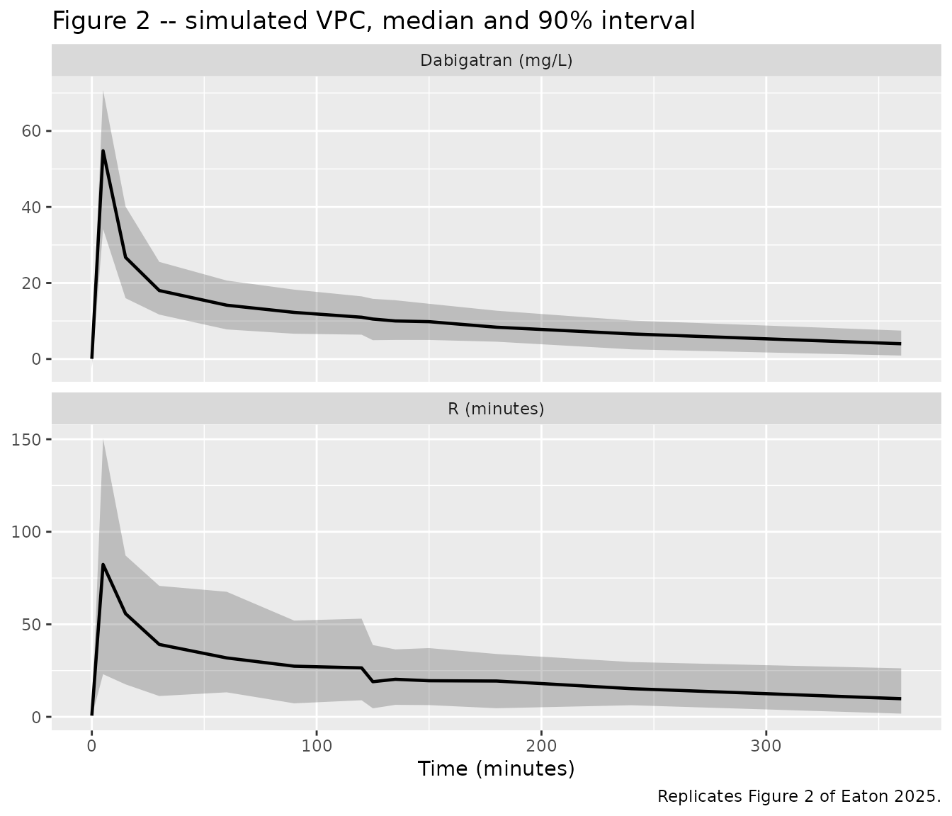

Read off the published Figure 2, observed dabigatran concentrations peak near 55 mg/L at 5 min and fall to a few mg/L by 480 min, while R-times peak near 100 min at 5 min and fall to under 10 min by 480 min. The landmarks below are the typical-value trajectory at the median study weight.

typ <- rxode2::zeroRe(mod)
#> ℹ parameter labels from comments will be replaced by 'label()'

# 480 min is a landmark of the published figure but is not one of the study's
# sampling times, so it is added to the typical-value grid.
typ_events <- make_events(tibble(id = 1L, WT = wt_typical),
                          sort(unique(c(samp_times, 480))))
sim_typ <- rxode2::rxSolve(typ, typ_events, keep = c("WT", "endpoint"),
                           useLinCmt = FALSE) |>
  as.data.frame()
#> ℹ omega/sigma items treated as zero: 'etalcl', 'etalvc', 'etalq', 'etalvp', 'etale0', 'etalec50', 'etalkel_ida'

sim_typ |>
  filter(endpoint == "Cc", time %in% c(5, 60, 120, 240, 480)) |>
  transmute(time, Cc = round(Cc, 2), Rtime = round(Rtime, 1)) |>
  rename("Time (min)" = time,
         "Dabigatran (mg/L)" = Cc,
         "R-time (min)" = Rtime) |>
  knitr::kable(caption = paste(
    "Typical-value trajectory at the median study weight",
    paste0("(", wt_typical, " kg), including idarucizumab at 120 min.")
  ))

Typical-value trajectory at the median study weight (33.9 kg), including idarucizumab at 120 min.
Time (min)	Dabigatran (mg/L)	R-time (min)
5	55.97	89.2
60	14.62	34.2
120	11.52	28.2
240	7.16	18.2
480	2.77	8.2


# Hold the trajectory to the Figure 2 landmarks read off the published panels.
landmark <- function(t, what) {
  sim_typ[[what]][sim_typ$endpoint == "Cc" & sim_typ$time == t]
}
stopifnot(
  abs(landmark(5, "Cc") - 55) < 10,        # peak dabigatran near 55 mg/L
  landmark(480, "Cc") < 5,                 # a few mg/L by 480 min
  abs(landmark(5, "Rtime") - 100) < 20,    # peak R-time near 100 min
  landmark(480, "Rtime") < 10              # under 10 min by 480 min
)

Figure 3 – concentration-response for R-time

Figure 3 of Eaton 2025 plots R-time against dabigatran effect-site concentration and states that an R-time of 13 min (normal range 4-8 min) is a suitable target effect, corresponding to a target concentration of 5 mg/L. The curve below is traced parametrically from the typical-value simulation, so it is computed by the packaged model rather than re-derived here.

# Replicates Figure 3 of Eaton 2025: R-time vs effect-site concentration.
# Simulated without idarucizumab so that Rtime is the pure Emax response.
ce_events <- make_events(tibble(id = 1L, WT = wt_typical),
                         seq(0, 480, by = 1), idarucizumab = FALSE)
sim_ce <- rxode2::rxSolve(typ, ce_events, keep = c("WT", "endpoint"),
                          useLinCmt = FALSE) |>
  as.data.frame() |>
  filter(endpoint == "Cc")
#> ℹ omega/sigma items treated as zero: 'etalcl', 'etalvc', 'etalq', 'etalvp', 'etale0', 'etalec50', 'etalkel_ida'

ggplot(sim_ce, aes(Ce, Rtime)) +
  geom_line(linewidth = 0.8) +
  geom_point(
    data = data.frame(Ce = 5, Rtime = 13),
    colour = "firebrick", size = 3, shape = 4, stroke = 1.2
  ) +
  labs(x = "Effect-site concentration (mg/L)", y = "R-time (minutes)",
       title = "Figure 3 -- concentration-response for R-time",
       caption = paste("Replicates Figure 3 of Eaton 2025.",
                       "The cross marks the published target",
                       "(5 mg/L, R-time 13 min)."))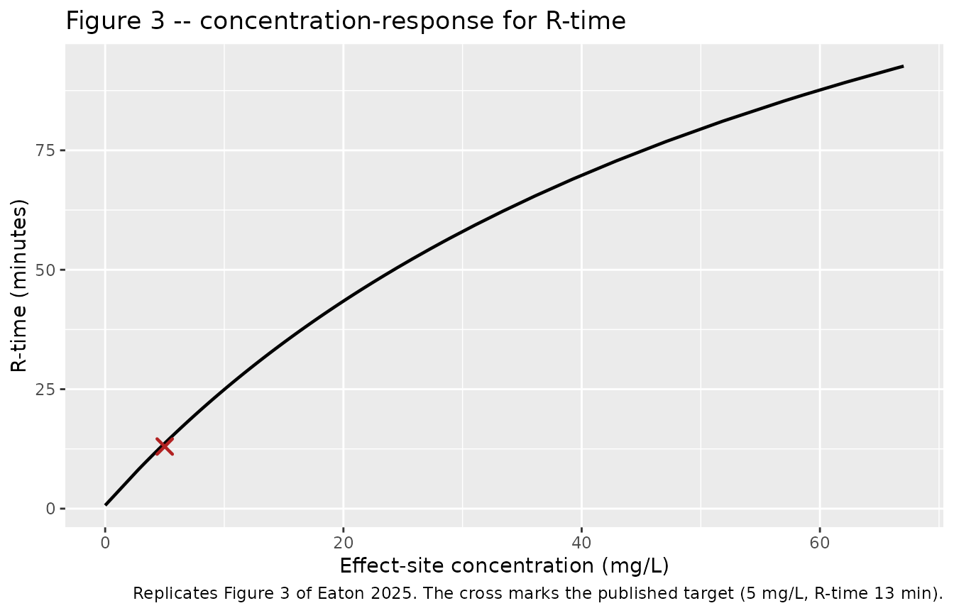

# Post-peak branch is monotone in Ce, so interpolation is well defined.
decline <- sim_ce |> filter(time >= 10) |> arrange(Ce)
rtime_at_target <- approx(decline$Ce, decline$Rtime, xout = 5)$y

cat(sprintf(
  "R-time at an effect-site concentration of 5 mg/L: %.2f min (Eaton 2025 Figure 3: 13 min)\n",
  rtime_at_target
))
#> R-time at an effect-site concentration of 5 mg/L: 13.69 min (Eaton 2025 Figure 3: 13 min)

# The published target is quoted to whole minutes, so agreement to within
# 1 min is the tightest assertion the source supports.
stopifnot(abs(rtime_at_target - 13) < 1)

Figure 4 – target-concentration dosing regimen

Figure 4 simulates a loading dose of dabigatran 0.25 mg/kg followed by a maintenance infusion of 0.0175 mg/kg/min for 30 min and then 0.0075 mg/kg/min from 30 to 90 min, and reports that this achieves a steady-state target concentration of 5 mg/L. The published simulation additionally carries a cardiopulmonary-bypass circuit compartment that is pre-loaded to the same 5 mg/L target; because it starts at the target concentration there is no net drug flux into it, so the two-compartment model reproduces the profile.

The loading dose is given here as a 1-min infusion, matching how dabigatran was administered in the study itself; the article does not state a loading-dose duration. The choice does not affect the peak, since 0.25 mg/kg delivered into a central volume of 2.94 L/70 kg gives 5.95 mg/L whether it is infused over 1 min or given as a bolus.

# Replicates Figure 4 of Eaton 2025, simulated at the 70 kg standard weight.
wt_std <- 70
regimen <- bind_rows(
  data.frame(id = 1L, WT = wt_std, time =  0, amt = 0.25   * wt_std,
             evid = 1L, rate = 0.25 * wt_std / 1,  cmt = "central", dvid = NA_integer_),
  data.frame(id = 1L, WT = wt_std, time =  0, amt = 0.0175 * wt_std * 30,
             evid = 1L, rate = 0.0175 * wt_std,    cmt = "central", dvid = NA_integer_),
  data.frame(id = 1L, WT = wt_std, time = 30, amt = 0.0075 * wt_std * 60,
             evid = 1L, rate = 0.0075 * wt_std,    cmt = "central", dvid = NA_integer_),
  data.frame(id = 1L, WT = wt_std, time = seq(0, 150, by = 0.5),
             amt = NA_real_, evid = 0L, rate = NA_real_,
             cmt = NA_character_, dvid = 1L)
)
regimen <- regimen[order(regimen$time, -regimen$evid), ]

sim_reg <- rxode2::rxSolve(typ, regimen, keep = "WT", useLinCmt = FALSE) |>
  as.data.frame()
#> ℹ omega/sigma items treated as zero: 'etalcl', 'etalvc', 'etalq', 'etalvp', 'etale0', 'etalec50', 'etalkel_ida'

ggplot(sim_reg, aes(time, Cc)) +
  geom_line(linewidth = 0.8) +
  geom_hline(yintercept = 5, linetype = "dashed", colour = "firebrick") +
  coord_cartesian(ylim = c(0, 7)) +
  labs(x = "Time (minutes)", y = "Concentration (mg/L)",
       title = "Figure 4 -- loading dose plus maintenance infusions",
       caption = paste("Replicates Figure 4 of Eaton 2025.",
                       "Dashed line: 5 mg/L target concentration."))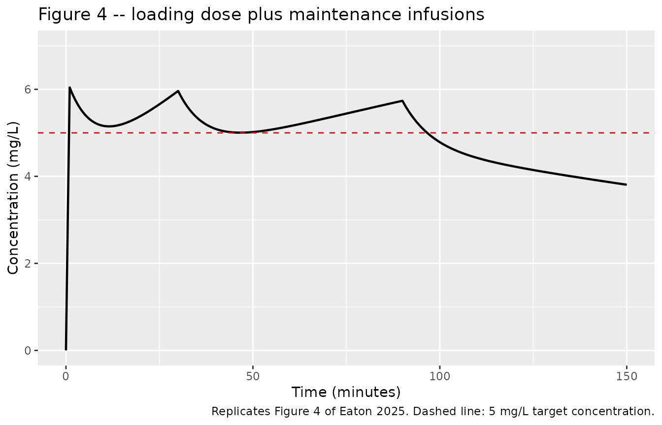

# Assess the maintenance window, i.e. from the end of the 1-min loading
# infusion to the end of the 90-min bypass period.
bypass_window <- sim_reg |> filter(time >= 1, time <= 90)

cat(sprintf(
  "Concentration over the 1-90 min maintenance window: %.2f-%.2f mg/L (mean %.2f); target 5 mg/L\n",
  min(bypass_window$Cc), max(bypass_window$Cc), mean(bypass_window$Cc)
))
#> Concentration over the 1-90 min maintenance window: 5.00-6.04 mg/L (mean 5.36); target 5 mg/L

# The published regimen holds the concentration at or just above the 5 mg/L
# target for the whole bypass period. The peak occurs at the end of the loading
# dose and is inherent to the published numbers: 0.25 mg/kg into a central
# volume of 2.94 L/70 kg is 5.95 mg/L on its own, so a ~20% overshoot of the
# target is a property of the regimen rather than of this implementation.
stopifnot(
  min(bypass_window$Cc) > 4.9,                    # never falls below target
  max(bypass_window$Cc) < 6.1,                    # peak overshoot under 22%
  abs(mean(bypass_window$Cc) - 5) / 5 < 0.10      # window average within 10%
)

# The loading dose alone, as an instantaneous input into the central volume.
stopifnot(abs(0.25 * wt_std / 2.94 - 5.95) < 0.01)

Supplementary Figure S1 – idarucizumab reversal

Eaton 2025 reports that idarucizumab 15 mg/kg given 120 min after dabigatran reduced R-time “by approximately 5 min over the 5 min after administration”, and in the Discussion that the reversal agent reduced reaction time by 30%.

# Replicates Supplementary Figure S1 of Eaton 2025.
s1_events <- make_events(tibble(id = 1L, WT = wt_typical), seq(0, 300, by = 1))
s1_no     <- make_events(tibble(id = 1L, WT = wt_typical), seq(0, 300, by = 1),
                         idarucizumab = FALSE)

s1 <- bind_rows(
  rxode2::rxSolve(typ, s1_events, keep = c("WT", "endpoint"), useLinCmt = FALSE) |>
    as.data.frame() |> mutate(arm = "With idarucizumab"),
  rxode2::rxSolve(typ, s1_no, keep = c("WT", "endpoint"), useLinCmt = FALSE) |>
    as.data.frame() |> mutate(arm = "Dabigatran alone")
) |>
  filter(endpoint == "Cc")
#> ℹ omega/sigma items treated as zero: 'etalcl', 'etalvc', 'etalq', 'etalvp', 'etale0', 'etalec50', 'etalkel_ida'
#> ℹ omega/sigma items treated as zero: 'etalcl', 'etalvc', 'etalq', 'etalvp', 'etale0', 'etalec50', 'etalkel_ida'

ggplot(s1, aes(time, Rtime, colour = arm)) +
  geom_line(linewidth = 0.8) +
  geom_vline(xintercept = 120, linetype = "dotted") +
  labs(x = "Time (minutes)", y = "R-time (minutes)", colour = NULL,
       title = "Supplementary Figure S1 -- effect of idarucizumab on R-time",
       caption = "Replicates Supplementary Figure S1 of Eaton 2025.")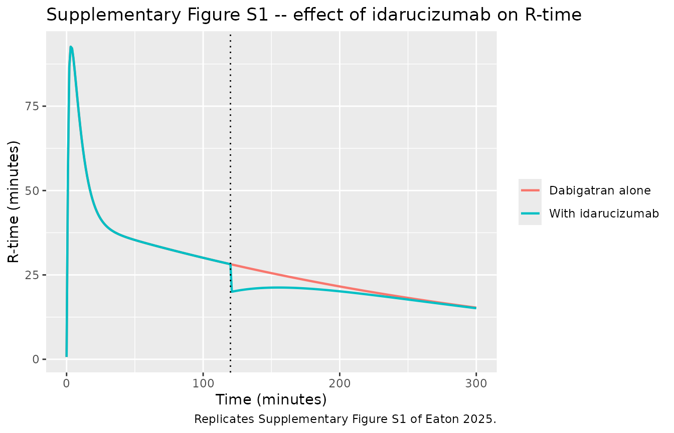

s1_wide <- s1 |>
  select(time, arm, Rtime) |>
  tidyr::pivot_wider(names_from = arm, values_from = Rtime) |>
  mutate(reduction = `Dabigatran alone` - `With idarucizumab`,
         pct = 100 * reduction / `Dabigatran alone`)

s1_wide |>
  filter(time %in% c(121, 125, 150, 180, 240)) |>
  transmute(time,
            `Dabigatran alone` = round(`Dabigatran alone`, 1),
            `With idarucizumab` = round(`With idarucizumab`, 1),
            reduction = round(reduction, 2),
            pct = round(pct, 1)) |>
  rename("Time (min)" = time,
         "R-time reduction (min)" = reduction,
         "Reduction (%)" = pct) |>
  knitr::kable(caption = "Model-predicted idarucizumab effect on R-time.")

Model-predicted idarucizumab effect on R-time.
Time (min)	Dabigatran alone	With idarucizumab	R-time reduction (min)	Reduction (%)
121	28.1	20.0	8.07	28.7
125	27.7	20.3	7.40	26.7
150	25.5	21.2	4.29	16.8
180	23.1	20.9	2.23	9.7
240	18.8	18.2	0.60	3.2


peak <- s1_wide |> filter(time == 125)
cat(sprintf(
  "At 5 min after idarucizumab the model predicts a %.1f min (%.0f%%) reduction in R-time; Eaton 2025 reports about 5 min and, in the Discussion, 30%%.\n",
  peak$reduction, peak$pct
))
#> At 5 min after idarucizumab the model predicts a 7.4 min (27%) reduction in R-time; Eaton 2025 reports about 5 min and, in the Discussion, 30%.

PKNCA validation

The source paper reports no non-compartmental analysis, so there is no published NCA table to compare against. Instead, NCA of the simulated dabigatran profile is checked against the identities implied by the published parameters themselves: AUC0-inf must equal Dose / CL for every subject, and the terminal half-life must equal ln(2) / beta, where beta is the smaller eigenvalue of the two-compartment system built from the published CL, V1, Q and V2. This is a non-circular check of the ODE encoding against the standard two-compartment analytic solution.

nca_times <- unique(c(seq(0, 10, by = 0.25), seq(10, 60, by = 1),
                      seq(60, 360, by = 5), seq(360, 1440, by = 20)))

nca_events <- make_events(cohort, nca_times, idarucizumab = FALSE) |>
  filter(evid == 1L | dvid == 1L)

sim_nca_raw <- rxode2::rxSolve(mod, nca_events, keep = c("WT", "endpoint"),
                               useLinCmt = FALSE) |>
  as.data.frame()

stopifnot(dplyr::n_distinct(sim_nca_raw$id) == n_sheep)
stopifnot(all(sim_nca_raw$Cc >= 0))

sim_nca <- sim_nca_raw |>
  filter(!is.na(Cc)) |>
  mutate(treatment = "Dabigatran 4 mg/kg IV") |>
  select(id, time, Cc, treatment)

# Guarantee a time-zero record per subject (IV infusion: pre-dose Cc = 0).
sim_nca <- bind_rows(
  sim_nca,
  sim_nca |> distinct(id, treatment) |> mutate(time = 0, Cc = 0)
) |>
  distinct(id, treatment, time, .keep_all = TRUE) |>
  arrange(id, treatment, time)

dose_df <- nca_events |>
  filter(evid == 1L) |>
  mutate(treatment = "Dabigatran 4 mg/kg IV") |>
  select(id, time, amt, treatment)

conc_obj <- PKNCA::PKNCAconc(sim_nca, Cc ~ time | treatment + id,
                             concu = "mg/L", timeu = "min")
dose_obj <- PKNCA::PKNCAdose(dose_df, amt ~ time | treatment + id,
                             doseu = "mg")

intervals <- data.frame(
  start      = 0,
  end        = Inf,
  cmax       = TRUE,
  tmax       = TRUE,
  aucinf.obs = TRUE,
  half.life  = TRUE
)

nca_res <- PKNCA::pk.nca(PKNCA::PKNCAdata(conc_obj, dose_obj, intervals = intervals))

Per-subject analytic identities

# Per-subject individual parameters as the model actually computed them.
subj_par <- sim_nca_raw |>
  group_by(id) |>
  summarise(WT = first(WT), cl = first(cl), vc = first(vc),
            q = first(q), vp = first(vp), .groups = "drop") |>
  mutate(dose = 4 * WT)

# Closed-form two-compartment quantities from the individual micro-constants.
two_cmt_ref <- function(dose, dur, cl, vc, q, vp) {
  k10 <- cl / vc
  k12 <- q / vc
  k21 <- q / vp
  s <- k10 + k12 + k21
  disc <- sqrt(s^2 - 4 * k10 * k21)
  alpha <- (s + disc) / 2
  beta <- (s - disc) / 2
  a <- (alpha - k21) / (alpha - beta)
  b <- (k21 - beta) / (alpha - beta)
  r0 <- dose / dur
  tibble(
    cmax_ref = (r0 / vc) * (a / alpha * (1 - exp(-alpha * dur)) +
                              b / beta * (1 - exp(-beta * dur))),
    aucinf_ref = dose / cl,
    halflife_ref = log(2) / beta
  )
}

ref <- subj_par |>
  rowwise() |>
  mutate(two_cmt_ref(dose, 1, cl, vc, q, vp)) |>
  ungroup()

nca_wide <- as.data.frame(nca_res$result) |>
  select(id, PPTESTCD, PPORRES) |>
  tidyr::pivot_wider(names_from = PPTESTCD, values_from = PPORRES) |>
  mutate(id = as.integer(as.character(id)))

check <- ref |>
  left_join(nca_wide, by = "id") |>
  mutate(
    auc_err  = abs(aucinf.obs - aucinf_ref) / aucinf_ref,
    cmax_err = abs(cmax - cmax_ref) / cmax_ref,
    hl_err   = abs(half.life - halflife_ref) / halflife_ref
  )

stopifnot(nrow(check) == n_sheep, !anyNA(check$auc_err))

cat(sprintf("Worst per-subject relative error across %d sheep:\n", n_sheep))
#> Worst per-subject relative error across 100 sheep:
cat(sprintf("  AUC0-inf vs Dose/CL      : %.3f%%\n", 100 * max(check$auc_err)))
#>   AUC0-inf vs Dose/CL      : 0.024%
cat(sprintf("  Cmax vs analytic infusion: %.3f%%\n", 100 * max(check$cmax_err)))
#>   Cmax vs analytic infusion: 0.000%
cat(sprintf("  t1/2 vs ln(2)/beta       : %.3f%%\n", 100 * max(check$hl_err)))
#>   t1/2 vs ln(2)/beta       : 0.407%

# Tightened to the accuracy actually achieved; these are exact identities, so
# the only residual is numerical (ODE tolerance and the NCA time grid).
stopifnot(max(check$auc_err)  < 0.01)
stopifnot(max(check$cmax_err) < 0.01)
stopifnot(max(check$hl_err)   < 0.01)

Comparison against the analytic reference

reference <- tibble::tibble(
  treatment   = "Dabigatran 4 mg/kg IV",
  cmax        = median(ref$cmax_ref),
  tmax        = 1,                       # end of the 1-min infusion
  aucinf.obs  = median(ref$aucinf_ref),
  half.life   = median(ref$halflife_ref)
)

cmp <- nlmixr2lib::ncaComparisonTable(
  simulated = nca_res,
  reference = reference,
  by        = "treatment",
  units     = c(cmax = "mg/L", tmax = "min",
                aucinf.obs = "mg*min/L", half.life = "min"),
  tolerance_pct = 20
)

knitr::kable(
  cmp,
  caption = paste(
    "Simulated NCA vs the analytic two-compartment reference implied by the",
    "published parameters (cohort medians). * differs by >20%."
  ),
  align = c("l", "l", "r", "r", "r")
)

Simulated NCA vs the analytic two-compartment reference implied by the published parameters (cohort medians). * differs by >20%.
NCA parameter	treatment	Reference	Simulated	% diff
Cmax (mg/L)	Dabigatran 4 mg/kg IV	89.5	89.5	+0.0%
Tmax (min)	Dabigatran 4 mg/kg IV	1	1	+0.0%
AUC0-∞ (obs) (mg*min/L)	Dabigatran 4 mg/kg IV	5280	5280	+0.0%
t½ (min)	Dabigatran 4 mg/kg IV	189	189	-0.2%

No row exceeds the 20% tolerance: the packaged ODE system reproduces the closed-form two-compartment solution for the published parameters to well within numerical noise.

Assumptions and deviations

Residual-error scale. Tables 2 and 3 both print the proportional residual error under a “(%)” header. The pharmacodynamic row settles the convention: RUV PROP 37.0 can only be the fraction 0.370 (the supplementary control stream’s $THETA initial for RUV_CVPD is 0.412), so the pharmacokinetic row’s 0.47 is the fraction 0.0047, not 0.47. The supplement’s $THETA initial for RUV_CVCP is 0.0005, which is consistent with the smaller reading, and the width of the published Figure 2 prediction interval at 5 min is far too narrow for a 47% proportional error.
%BSV convention. Table 2 and Table 3 report %BSV, and the supplementary $OMEGA initial estimates show these are the approximate CV sqrt(omega^2) * 100 rather than the exact log-normal CV: Q 51.4% against an $OMEGA initial of 0.265 (0.514^2 = 0.264), V1 7.4% against 0.00591, Ce50 19.9% against 0.0395, E0 15.1% against 0.0227. The model therefore uses omega^2 = (%BSV / 100)^2.
Omega block structure not reproduced. The authors fitted $OMEGA BLOCK(4) across CL, V1, Q and V2 and $OMEGA BLOCK(2) across Ce50 and E0. Final off-diagonal estimates are not published – only the supplementary control stream’s initial covariances are available – so only the diagonal variances are encoded. Between-subject correlations are consequently absent from the simulated cohort.
etalvp fixed status. The supplementary $OMEGA BLOCK(4) carries PPVV2 with a FIX flag at 0.165 (40.6% BSV), while Table 2 reports 39.6%. The model uses the published Table 2 magnitude (0.396^2 = 0.156816) and retains the fixed() status the control stream documents. The two readings differ by one percentage point of BSV.
Hill coefficient. Table 3 reports N 1 FIX; the supplementary control stream’s $THETA (0.1,1.,8) for HILL carries no FIX flag. The published table is treated as authoritative and lhill is fixed.
Allometry on the equilibration half-time. The main text describes allometric scaling only for clearances (0.75) and volumes (1). The supplementary $PK block also scales TEQ (the plasma-effect equilibration half-time) by FSZT = (WT/70)**0.25, which the model encodes as an exponent of -0.25 on ke0. This exponent is sourced from the supplement, not from the article text.
Idarucizumab dosing convention. The reversal agent is modelled exactly as published: a unit dose (amt = 1) into depot_kpd represents one 15 mg/kg idarucizumab administration, so lslope_ida carries units of minutes per unit dose. No idarucizumab concentrations were measured and no dose range was explored, so the model cannot be extrapolated to other idarucizumab doses.
Magnitude of the reversal effect. The model predicts an R-time reduction of 7.4 min (27%) at 5 min after idarucizumab, and 8.1 min (29%) at 1 min after it, when the K-PD compartment is fullest. That matches the Discussion’s “reducing reaction time by 30%” but is larger than the “approximately 5 min” quoted in the Results, which describes the observed trace in Supplementary Figure S1 for a single animal rather than the population prediction.
R-time can go negative. The published structure subtracts the idarucizumab effect from the sigmoid Emax effect with no lower bound, so large depot_kpd amounts combined with low effect-site concentrations can drive predicted R-time below zero. This is a property of the published model, reproduced faithfully rather than patched.
The published regimen overshoots its own target. Reproducing the Figure 4 regimen with the Table 2 parameters holds the concentration between 5.0 and 6.0 mg/L across the 90-min bypass window, i.e. at or above the stated 5 mg/L target rather than centred on it. The excess is arithmetic: the loading dose of 0.25 mg/kg divided by the central volume of 2.94 L/70 kg is 5.95 mg/L before the maintenance infusion contributes anything. The published Figure 4 additionally carries the bypass-circuit compartment (below), whose extra volume would draw the peak down; that compartment cannot be reproduced because V3 is not reported.
Cardiopulmonary-bypass circuit model not packaged. The “Determination of dabigatran dose” section prints a third structure – a Berkeley Madonna simulation adding a bypass-circuit compartment exchanging with the central compartment at pump flow Q3 and holding circuit volume V3. Neither Q3 nor V3 is reported anywhere in the article or its supplement (Supplementary Figure S2 is a diagram only). The printed circuit equation d/dt(CPB) = C1*Q2 - C3*Q3 is also internally inconsistent: the flux from the central compartment into the circuit should be carried by the pump flow Q3, not by the intercompartmental clearance Q2. Because the circuit is pre-loaded to the target concentration there is no net flux into it, so Figure 4 is reproducible from the two-compartment model alone, as shown above. No values were invented for Q3 or V3.
Target R-time quoted inconsistently. Figure 3’s caption gives an R-time target of 13 min for a 5 mg/L target concentration; the Discussion says 16 min. The published Emax parameters give 0.681 + 180 * 5 / (64.2 + 5) = 13.7 min, so the Figure 3 value is the self-consistent one and is used here.
Virtual cohort. Body weights are drawn uniformly across the 28.7-41.8 kg range of Table 1 rather than resampled from the five observed animals, so the simulated weight distribution is broader than the study’s.