Tofacitinib exposure-response in psoriatic arthritis (Menon 2025)
Source:vignettes/articles/Menon_2025_tofacitinib.Rmd
Menon_2025_tofacitinib.RmdModel and source
- Citation: Menon S, Shoji S, Tsuchiwata S, Fallon L, Kanik K. Exposure-Response Analysis of Tofacitinib in Active Psoriatic Arthritis: Results from Two Phase 3 Studies. J Clin Pharmacol. 2025;65(3):369-377.
- Article (open access): https://doi.org/10.1002/jcph.6147
- Supporting information (Figures S1 and S2, hemoglobin visual predictive checks) is distributed with the article.
Menon 2025 pools the two phase 3 psoriatic arthritis (PsA) trials
OPAL Broaden (TNF-inhibitor naive) and OPAL Beyond (TNF-inhibitor
experienced) and fits three independent exposure-response models, each
driven by the patient’s own steady-state average tofacitinib
concentration (Cavg) predicted from the PsA population PK model of Xie
2019 (modellib("Xie_2019_tofacitinib")). Each is packaged
as its own model file:
| Model file | Endpoint | Structure | Software |
|---|---|---|---|
Menon_2025_tofacitinib_acr |
ACR20 / ACR50 / ACR70 at Month 3 | four-category ordered-categorical logit, Emax in Cavg | SAS PROC NLMIXED |
Menon_2025_tofacitinib_hb |
hemoglobin time course | indirect response, Cavg stimulates loss | NONMEM 7.3 |
Menon_2025_tofacitinib_hb_decrease |
hemoglobin decrease > 2 g/dL | logistic regression, linear in Cavg | NONMEM 7.3 |
None of the three carries a PK layer: the exposure enters as the
covariate column CAV (ng/mL), 0 for placebo.
mod_acr <- rxode2::rxode(readModelDb("Menon_2025_tofacitinib_acr"))
mod_hb <- rxode2::rxode(readModelDb("Menon_2025_tofacitinib_hb"))
#> ℹ parameter labels from comments will be replaced by 'label()'
mod_dec <- rxode2::rxode(readModelDb("Menon_2025_tofacitinib_hb_decrease"))

ini_est <- function(ui) {
  d <- ui$iniDf
  stats::setNames(d$est, d$name)
}
p_acr <- ini_est(mod_acr)
p_hb <- ini_est(mod_hb)
p_dec <- ini_est(mod_dec)
Population
The ACR analysis used 655 patients with a Month-3 ACR assessment and an individual Cavg (OPAL Broaden 298, OPAL Beyond 357; 15 of the 670 randomised to placebo or tofacitinib had no Cavg, Table 1 footnote b). The hemoglobin analyses used 685 patients (309 male, 376 female) with median weight 83 kg, median age 50 years and median baseline hemoglobin 13.8 g/dL (Results). Patients had active PsA by the CASPAR criteria with at least 3 swollen and 3 tender joints and active plaque psoriasis, on a stable background conventional synthetic DMARD (predominantly methotrexate, sulfasalazine or leflunomide), and were randomised to placebo or tofacitinib 5 or 10 mg twice daily; placebo patients advanced blinded to tofacitinib at Month 3, so placebo hemoglobin data stop at Month 3 while active arms run to Month 6 or 12. The adalimumab arm of OPAL Broaden is not analysed.
Median (range) Cavg was 17.6 (6.67-47.2) ng/mL at 5 mg and 36.1 (15.1-88.1) ng/mL at 10 mg twice daily (Results).
Source trace
| Quantity | Value | Source |
|---|---|---|
| ACR model equation | logit Pr(sACR >= m) = Int - I(m>=2) exp(theta2) - I(m>=3) exp(theta3) + Emax Cavg / (Cavg + exp(theta5)) |
Methods, ACR equation |
logit_bl_acr20 (Int, theta1) |
-0.852 | Table 2 |
lgap_acr50 (theta2) |
-0.0636 (exp 0.938) | Table 2 |
lgap_acr70 (theta3) |
-0.201 (exp 0.818) | Table 2 |
emax_acr (theta4) |
1.76 logit | Table 2 |
lec50_acr (theta5) |
2.84 (EC50 17.1 ng/mL) | Table 2 |
| Hemoglobin equation |
dR/dt = kin - kout R EFF,
EFF = 1 + Cavg / C',
R(0) = R0 = kin / kout
|
Methods, hemoglobin equations |
lrbase (R0) |
log(13.8 g/dL) | Table 3 |
lkout |
log(0.014 1/day) | Table 3 |
lcprime (C’) |
log(1670 ng/mL) | Table 3 |
etalrbase |
0.0881^2 (printed variance 0.008) | Table 3 and footnote a |
etalcprime |
0.99^2 (printed variance 0.980, on 1/C’) | Table 3 and footnote a |
expSd |
0.0381 (log-scale additive) | Table 3 ‘RV (CV)’ 3.81%; Methods residual equation |
| Logistic equation | logit Pr(Y = 1) = theta0 + theta_cov Cavg |
Methods, hemoglobin-decrease equation |
logit_ref (theta0) |
-4.168 | back-solved, see below; not printed |
e_cav_logit (theta_cov) |
0.03105 per ng/mL | back-solved, see below; not printed |
Virtual cohort
Each arm has 200 patients. The paper’s individual Cavg values are not published, so the cohort draws them log-normally around the printed arm medians with the 31.7% inter-individual variability of CL/F in Xie 2019 (Table 3), the source of the paper’s Cavg. With that spread the simulated ranges are similar to the printed ones.
set.seed(20251)
n_arm <- 200L
omega_cl <- 0.317
cohort <- tibble::tibble(
  arm = factor(rep(c("Placebo", "5 mg BID", "10 mg BID"), each = n_arm),
               levels = c("Placebo", "5 mg BID", "10 mg BID")),
  id = seq_len(3L * n_arm)
) |>
  mutate(
    cav_median = c(Placebo = 0, `5 mg BID` = 17.6, `10 mg BID` = 36.1)[as.character(arm)],
    CAV = cav_median * exp(stats::rnorm(dplyr::n(), 0, omega_cl))
  )

cohort |>
  filter(arm != "Placebo") |>
  group_by(arm) |>
  summarise(median = median(CAV), min = min(CAV), max = max(CAV), .groups = "drop") |>
  dplyr::rename("Arm" = arm, "Median Cavg (ng/mL)" = median,
                "Min" = min, "Max" = max) |>
knitr::kable(digits = 1, caption = "Simulated Cavg; paper: 17.6 (6.67-47.2) and 36.1 (15.1-88.1) ng/mL.")| Arm | Median Cavg (ng/mL) | Min | Max |
|---|---|---|---|
| 5 mg BID | 17.3 | 7.0 | 35.6 |
| 10 mg BID | 34.7 | 13.6 | 70.0 |
Cavg from the upstream population PK model
The CAV column is an output of a PK model, not a dose.
PKNCA on a steady-state dosing interval of
Xie_2019_tofacitinib (typical non-Hispanic White male, 83.3
kg, 50 years) recovers Cavg as AUCtau / tau and shows where the paper’s
medians sit relative to that patient.
mod_pk <- rxode2::rxode(readModelDb("Xie_2019_tofacitinib"))
#> ℹ parameter labels from comments will be replaced by 'label()'
tau <- 12
ev_pk <- lapply(c(5, 10), function(dose) {
  rxode2::et(amt = dose, ii = tau, addl = 27, cmt = "depot") |>
    rxode2::et(seq(0, 28 * tau, by = 0.1), cmt = "central") |>
    as.data.frame() |>
    mutate(dose = dose)
})
ev_pk <- bind_rows(ev_pk[[1]] |> mutate(id = 1L), ev_pk[[2]] |> mutate(id = 2L)) |>
  mutate(AGE = 50, WT = 83.3, CRCL_BASE = 120, CRP = 0.49, SEXF = 0,
         RACE_BLACK = 0, RACE_ASIAN = 0, RACE_OTHER = 0, RACE_HISPANIC = 0)

sim_pk <- rxode2::rxSolve(rxode2::zeroRe(mod_pk), ev_pk, returnType = "data.frame") |>
  left_join(data.frame(id = 1:2, dose = c(5, 10)), by = "id") |>
  mutate(treatment = paste(dose, "mg BID"))
#> Warning: No sigma parameters in the model
#> ℹ omega/sigma items treated as zero: 'etalcl', 'etalka', 'etaruv'
#> Warning: multi-subject simulation without without 'omega'

conc_pk <- sim_pk |>
  filter(!is.na(Cc)) |>
  select(id, time, Cc, treatment) |>
  bind_rows(sim_pk |> distinct(id, treatment) |> mutate(time = 0, Cc = 0)) |>
  distinct(id, time, .keep_all = TRUE) |>
  arrange(id, time)
dose_pk <- ev_pk |>
  filter(evid == 1) |>
  mutate(treatment = paste(dose, "mg BID")) |>
  select(id, time, amt, treatment)
# Cc is in ng/mL with doses in mg (Xie 2019 units), so AUC is ng*h/mL.
o_conc <- PKNCA::PKNCAconc(conc_pk, Cc ~ time | treatment + id)
o_dose <- PKNCA::PKNCAdose(dose_pk, amt ~ time | treatment + id)
intervals <- data.frame(start = 27 * tau, end = 28 * tau, cav = TRUE, cmax = TRUE)
nca <- as.data.frame(PKNCA::pk.nca(PKNCA::PKNCAdata(o_conc, o_dose, intervals = intervals)))

cav_nca <- nca |>
  filter(PPTESTCD == "cav") |>
  select(treatment, PPORRES)
cl_typ <- exp(ini_est(mod_pk)[["lcl"]]) * ini_est(mod_pk)[["e_race_hispanic_cl"]]
cav_nca <- cav_nca |>
  mutate(
    dose = as.numeric(sub(" mg BID", "", treatment)),
    closed_form = dose * 1000 / (cl_typ * tau),
    paper_median = c(17.6, 36.1)[match(dose, c(5, 10))]
  )
cav_nca |>
  arrange(dose) |>
  select(treatment, PPORRES, closed_form, paper_median) |>
  dplyr::rename("Regimen" = treatment, "PKNCA Cavg (ng/mL)" = PPORRES,
                "Dose / (CL/F tau)" = closed_form,
                "Paper median Cavg" = paper_median) |>
knitr::kable(digits = 2)| Regimen | PKNCA Cavg (ng/mL) | Dose / (CL/F tau) | Paper median Cavg |
|---|---|---|---|
| 5 mg BID | 18.19 | 18.24 | 17.6 |
| 10 mg BID | 36.39 | 36.47 | 36.1 |
# The NCA and the closed form use the same solved profile, so they agree to
# trapezoidal error on a 0.1 h grid.
stopifnot(all(abs(cav_nca$PPORRES / cav_nca$closed_form - 1) < 0.01))
The typical patient’s Cavg (36.4 and 18.2 ng/mL) is 2% above the paper’s medians; the medians are over the trial population’s covariates and CL/F random effects.
ACR response at Month 3
Typical predictions
solve_acr <- function(cav) {
  ev <- data.frame(id = seq_along(cav), time = 0, evid = 0L, amt = NA_real_, dv = NA_real_, CAV = cav)
  rxode2::rxSolve(rxode2::zeroRe(mod_acr), ev, returnType = "data.frame")
}
acr_tv <- solve_acr(c(0, 17.6, 36.1)) |>
  mutate(arm = c("Placebo", "5 mg BID", "10 mg BID"))
#> Warning: No omega parameters in the model
#> Warning: multi-subject simulation without without 'omega'

acr_cmp <- tibble::tibble(
  arm = rep(acr_tv$arm, each = 3),
  endpoint = rep(c("ACR20", "ACR50", "ACR70"), 3),
  model = 100 * c(t(as.matrix(acr_tv[, c("prob_acr20", "prob_acr50", "prob_acr70")]))),
  paper = c(30, 14, 7, 51, 29, 15, 58, 36, 20)
)
acr_cmp |>
  dplyr::rename("Arm" = arm, "Endpoint" = endpoint,
                "Model (%)" = model, "Menon 2025 (%)" = paper) |>
knitr::kable(digits = 1, caption = "Responder rates at Month 3 at the median Cavg per arm (Results, Predictive Checks).")| Arm | Endpoint | Model (%) | Menon 2025 (%) |
|---|---|---|---|
| Placebo | ACR20 | 29.9 | 30 |
| Placebo | ACR50 | 14.3 | 14 |
| Placebo | ACR70 | 6.9 | 7 |
| 5 mg BID | ACR20 | 51.0 | 51 |
| 5 mg BID | ACR50 | 28.9 | 29 |
| 5 mg BID | ACR70 | 15.2 | 15 |
| 10 mg BID | ACR20 | 58.5 | 58 |
| 10 mg BID | ACR50 | 35.5 | 36 |
| 10 mg BID | ACR70 | 19.6 | 20 |
# Typical-value algebra, no random draws: the printed rates are rounded to
# whole per cent.
stopifnot(all(abs(acr_cmp$model - acr_cmp$paper) < 0.6))

# Discussion: 51% and 68% of Emax at the 5 and 10 mg medians, and relative
# benefit 10 vs 5 mg of 1.14, 1.22, 1.27 for ACR20 / ACR50 / ACR70.
frac_emax <- c(17.6, 36.1) / (c(17.6, 36.1) + exp(p_acr[["lec50_acr"]]))
rel_benefit <- acr_cmp$model[acr_cmp$arm == "10 mg BID"] / acr_cmp$model[acr_cmp$arm == "5 mg BID"]
round(frac_emax, 3)
#> [1] 0.507 0.678
round(rel_benefit, 3)
#> [1] 1.146 1.227 1.283
# The model gives 1.146, 1.227 and 1.283: within 1% of the printed ratios,
# which the paper may have taken at slightly different Cavg values.
stopifnot(
  all(abs(frac_emax - c(0.51, 0.68)) < 0.006),
  all(abs(rel_benefit / c(1.14, 1.22, 1.27) - 1) < 0.015)
)
Exposure-response curves
Replicates the model-predicted lines of Figure 1 of Menon 2025.
cav_grid <- seq(0, 90, by = 0.5)
acr_curve <- solve_acr(cav_grid) |>
  mutate(CAV = cav_grid) |>
  select(CAV, prob_acr20, prob_acr50, prob_acr70) |>
  pivot_longer(-CAV, names_to = "endpoint", values_to = "p") |>
  mutate(endpoint = toupper(sub("prob_", "", endpoint)))
#> Warning: No omega parameters in the model
#> Warning: multi-subject simulation without without 'omega'

ggplot(acr_curve, aes(CAV, p)) +
  geom_line() +
  geom_vline(xintercept = c(17.6, 36.1), linetype = "dotted", colour = "steelblue") +
  facet_wrap(~endpoint) +
  scale_y_continuous(limits = c(0, 1)) +
  labs(x = "Cavg (ng/mL)", y = "Probability of response at Month 3",
       caption = "Replicates the predicted lines of Figure 1 of Menon 2025; dotted lines at the 5 and 10 mg BID median Cavg.")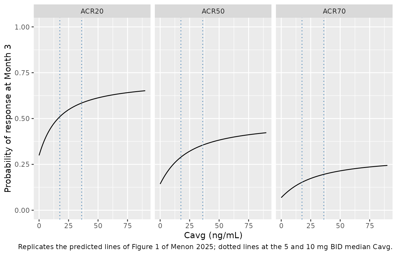
Simulated trial
The model is a joint ordered-categorical model, so a simulated patient falls in one of four categories and the three responder flags are nested. Drawing one uniform number per patient and comparing it with the three cumulative probabilities gives that.
acr_sim <- solve_acr(cohort$CAV) |>
  mutate(arm = cohort$arm, u = stats::runif(dplyr::n()),
         acr20 = u < prob_acr20, acr50 = u < prob_acr50, acr70 = u < prob_acr70)
#> Warning: No omega parameters in the model
#> Warning: multi-subject simulation without without 'omega'
stopifnot(all(acr_sim$acr70 <= acr_sim$acr50), all(acr_sim$acr50 <= acr_sim$acr20))

acr_sim |>
  group_by(arm) |>
  summarise(ACR20 = 100 * mean(acr20), ACR50 = 100 * mean(acr50),
            ACR70 = 100 * mean(acr70), .groups = "drop") |>
  dplyr::rename("Arm" = arm, "ACR20 (%)" = ACR20, "ACR50 (%)" = ACR50,
                "ACR70 (%)" = ACR70) |>
knitr::kable(digits = 1, caption = "Simulated responder rates, 200 patients per arm.")| Arm | ACR20 (%) | ACR50 (%) | ACR70 (%) |
|---|---|---|---|
| Placebo | 25.5 | 14.0 | 7.0 |
| 5 mg BID | 52.5 | 28.5 | 14.5 |
| 10 mg BID | 54.0 | 24.0 | 13.0 |
Hemoglobin time course
Closed-form check
Menon 2025 gives the on-drug solution
R(t) = R0 / EFF + R0 (1 - 1/EFF) exp(-kout EFF t). The ODE
in the model file is solved for the cohort with its own random effects,
and the closed form is evaluated with the same individual
parameters.
t_obs <- c(0, 14, 28, 56, 84, 112, 168, 252, 365)
ev_hb <- cohort |>
  select(id, arm, CAV) |>
  tidyr::expand_grid(time = t_obs) |>
  filter(!(arm == "Placebo" & time > 84)) |>
  mutate(evid = 0L, cmt = "hb") |>
  arrange(id, time)

rxode2::rxSetSeed(20252)
sim_hb <- rxode2::rxSolve(mod_hb, ev_hb, returnType = "data.frame",
                          atol = 1e-10, rtol = 1e-10) |>
  left_join(cohort |> select(id, arm), by = "id")

hb_check <- sim_hb |>
  mutate(closed = rbase / eff + rbase * (1 - 1 / eff) * exp(-exp(p_hb[["lkout"]]) * eff * time))
# Same drawn parameters on both sides, so the difference is solver error only.
stopifnot(max(abs(hb_check$hb - hb_check$closed)) < 1e-6)
Change from baseline at Month 3
Replicates the model-predicted rows of Table 4 of Menon 2025.
Following the paper’s Figure S2, the simulated change is
y_ij - BL_i, both values carrying residual error. Residual
error (3.81% of ~13.8 g/dL on each value) is large against the drug
effect and the drug slope has 99% CV, so the median change is pulled
toward the mean shift; the table therefore also shows the change without
residual error. Month 3 is taken as day 84.
cfb <- sim_hb |>
  group_by(id) |>
  mutate(bl_obs = sim[time == 0], bl_ipred = hb[time == 0]) |>
  ungroup() |>
  filter(time == 84) |>
  mutate(cfb_obs = sim - bl_obs, cfb_ipred = hb - bl_ipred)

cfb_tab <- cfb |>
  group_by(arm) |>
  summarise(median_obs = median(cfb_obs), median_ipred = median(cfb_ipred),
            mean_ipred = mean(cfb_ipred), .groups = "drop") |>
  mutate(paper = c(0.0, -0.2, -0.3), paper_ci = c("-0.1 to 0.1", "-0.3 to 0.0", "-0.4 to -0.2"))
cfb_tab |>
  dplyr::rename("Arm" = arm, "Median y - BL (g/dL)" = median_obs,
                "Median IPRED change" = median_ipred, "Mean IPRED change" = mean_ipred,
                "Menon 2025 median" = paper, "Menon 2025 95% CI" = paper_ci) |>
knitr::kable(digits = 2)| Arm | Median y - BL (g/dL) | Median IPRED change | Mean IPRED change | Menon 2025 median | Menon 2025 95% CI |
|---|---|---|---|---|---|
| Placebo | -0.07 | 0.00 | 0.00 | 0.0 | -0.1 to 0.1 |
| 5 mg BID | -0.16 | -0.11 | -0.19 | -0.2 | -0.3 to 0.0 |
| 10 mg BID | -0.35 | -0.20 | -0.33 | -0.3 | -0.4 to -0.2 |
A cohort of 200 per arm gives a noisy median of y - BL
(standard error about 0.07 g/dL), so the gate below uses a large base-R
Monte Carlo of the closed form with the model’s own parameters, which is
deterministic under set.seed().
set.seed(20253)
n_mc <- 20000L
mc <- lapply(c(0, 17.6, 36.1), function(med) {
  cav <- med * exp(stats::rnorm(n_mc, 0, omega_cl))
  r0 <- exp(p_hb[["lrbase"]] + stats::rnorm(n_mc, 0, sqrt(p_hb[["etalrbase"]])))
  cp <- exp(p_hb[["lcprime"]] + stats::rnorm(n_mc, 0, sqrt(p_hb[["etalcprime"]])))
  eff <- 1 + cav / cp
  r84 <- r0 / eff + r0 * (1 - 1 / eff) * exp(-exp(p_hb[["lkout"]]) * eff * 84)
  y0 <- r0 * exp(stats::rnorm(n_mc, 0, p_hb[["expSd"]]))
  y84 <- r84 * exp(stats::rnorm(n_mc, 0, p_hb[["expSd"]]))
  median(y84 - y0)
})
mc <- unlist(mc)
data.frame(Arm = c("Placebo", "5 mg BID", "10 mg BID"), MC = mc,
           Paper = c(0.0, -0.2, -0.3)) |>
  dplyr::rename("Monte Carlo median y - BL (g/dL)" = MC, "Menon 2025" = Paper) |>
knitr::kable(digits = 3)| Arm | Monte Carlo median y - BL (g/dL) | Menon 2025 |
|---|---|---|
| Placebo | 0.003 | 0.0 |
| 5 mg BID | -0.166 | -0.2 |
| 10 mg BID | -0.309 | -0.3 |
# Each Monte Carlo median rounds to the printed one-decimal value (within
# 0.05 g/dL; the 0.07 bound adds headroom for Monte Carlo error) and lies
# inside the printed 95% CI.
stopifnot(
  all(abs(mc - c(0.0, -0.2, -0.3)) < 0.07),
  mc[2] > -0.3, mc[2] < 0.0, mc[3] > -0.4, mc[3] < -0.2
)
sim_hb |>
  group_by(arm, time) |>
  summarise(p10 = quantile(sim, 0.1), p50 = median(sim), p90 = quantile(sim, 0.9),
            .groups = "drop") |>
  ggplot(aes(time, p50)) +
  geom_ribbon(aes(ymin = p10, ymax = p90), alpha = 0.25) +
  geom_line() +
  facet_wrap(~arm) +
  labs(x = "Time (day)", y = "Hemoglobin (g/dL)",
       caption = "Simulated median and 10th-90th percentiles; compare Figure S1 of Menon 2025.")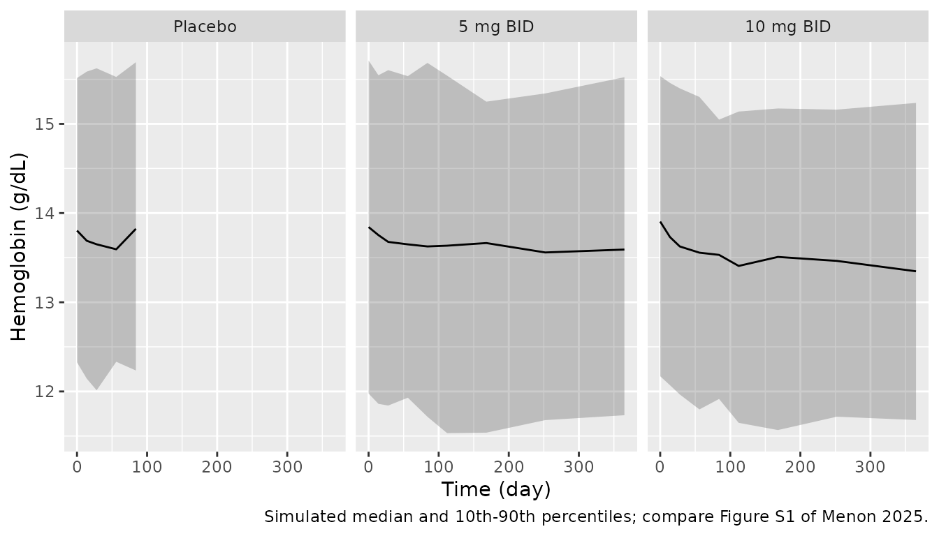
Hemoglobin decrease of more than 2 g/dL
The logistic intercept and slope are not printed. The paper prints the placebo-adjusted incidence at the 5 and 10 mg medians (1.08% at 17.6 ng/mL and 3.01% at 36.1 ng/mL) and the incidence at the 90th-percentile Cavg (7.97% at 54.8 ng/mL). The first two fix the two coefficients; the third is an independent check.
solve_dec <- function(cav) {
  ev <- data.frame(id = seq_along(cav), time = 0, evid = 0L, amt = NA_real_, dv = NA_real_, CAV = cav)
  rxode2::rxSolve(rxode2::zeroRe(mod_dec), ev, returnType = "data.frame")$prob_hb_decrease_2g
}
p <- solve_dec(c(0, 17.6, 36.1, 54.8))
#> Warning: No omega parameters in the model
#> Warning: multi-subject simulation without without 'omega'
dec_cmp <- data.frame(
  quantity = c("Placebo-adjusted, 5 mg median (17.6 ng/mL)",
               "Placebo-adjusted, 10 mg median (36.1 ng/mL)",
               "Incidence, 90th percentile Cavg (54.8 ng/mL)"),
  model = 100 * c(p[2] - p[1], p[3] - p[1], p[4]),
  paper = c(1.08, 3.01, 7.97)
)
dec_cmp |>
  dplyr::rename("Quantity" = quantity, "Model (%)" = model, "Menon 2025 (%)" = paper) |>
knitr::kable(digits = 2)| Quantity | Model (%) | Menon 2025 (%) |
|---|---|---|
| Placebo-adjusted, 5 mg median (17.6 ng/mL) | 1.08 | 1.08 |
| Placebo-adjusted, 10 mg median (36.1 ng/mL) | 3.01 | 3.01 |
| Incidence, 90th percentile Cavg (54.8 ng/mL) | 7.82 | 7.97 |
stopifnot(
  # Fitted conditions: reproduce to the printed two decimals.
  all(abs(dec_cmp$model[1:2] - dec_cmp$paper[1:2]) < 0.006),
  # Independent check: within 3% of the printed value.
  abs(dec_cmp$model[3] / dec_cmp$paper[3] - 1) < 0.03
)
Replicates the predicted line of Figure 2a of Menon 2025.
data.frame(CAV = cav_grid, p = solve_dec(cav_grid)) |>
  ggplot(aes(CAV, p)) +
  geom_line(colour = "navy") +
  geom_vline(xintercept = c(17.6, 25.9, 36.1), linetype = "dashed", colour = "grey50") +
  scale_y_continuous(limits = c(0, 0.5)) +
  labs(x = "Cavg (ng/mL)", y = "Incidence of decrease > 2 g/dL",
       caption = "Replicates the predicted line of Figure 2a of Menon 2025 (0.19 at 88 ng/mL).")
#> Warning: No omega parameters in the model
#> Warning: multi-subject simulation without without 'omega'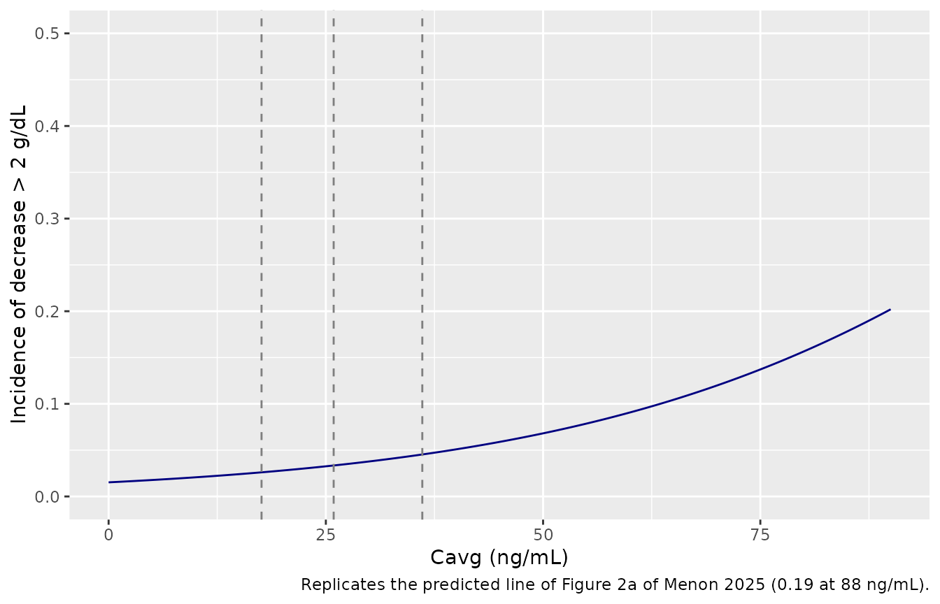
Assumptions and deviations
-
Logistic coefficients back-solved.
logit_refande_cav_logitinMenon_2025_tofacitinib_hb_decreaseare not printed. They are the exact solution of the two placebo-adjusted incidences printed at the 5 and 10 mg median Cavg. The resulting model predicts 7.82% at the printed 90th-percentile Cavg of 54.8 ng/mL where the paper prints 7.97% (1.9% low), and no pair of values within rounding of 1.08% and 3.01% reaches 7.97%, which suggests the medians used in the paper’s calculation were not exactly 17.6 and 36.1 ng/mL (“approximately”, Results). The curve also matches Figure 2a (about 0.015 at zero exposure and 0.19 at 88 ng/mL). -
IIV variances from the %CV footnote. Table 3 prints
the variances to one significant figure (0.008, 0.980) and the %CV
100 sqrt(omega^2)to three (8.81, 99.0); the model uses the squares of the latter (0.00776 and 0.980). -
IIV on 1/C’ carried on C’. The paper’s exponential
random effect is on the slope 1/C’. The model puts it on
lcprime; because the random effect is zero-mean normal,1/C' exp(eta)andC' exp(-eta)have the same distribution, so simulations are identical. -
Residual error. “log-transform on both sides …
additive error” with
theta_residualthe SD is rxode2’slnorm(expSd)withexpSd = 0.0381. - Cavg is constant from the first dose. The paper uses one Cavg per patient. Tofacitinib reaches steady state within a day, which is negligible against the 50-day hemoglobin turnover half-life.
- Placeholder residuals. The ACR and hemoglobin-decrease models are fitted by multinomial and Bernoulli likelihoods with no residual error; the fixed additive SD of 0.001 on each probability exists only so the model has an observation model.
-
Joint ACR outputs. The three probabilities are
cumulative,
prob_acr20 >= prob_acr50 >= prob_acr70always, and a joint simulation must draw one uniform per patient (as above), not three independent Bernoulli draws. -
Covariates not retained. Body weight on EC50 and
Emax and prior TNF inhibitor therapy on Int and Emax were tested (Table
1) and not retained; no estimates are printed. They are listed under
covariatesDataExcluded. - Virtual Cavg. Individual Cavg are drawn log-normally around the printed arm medians with the 31.7% CL/F variability of Xie 2019; the paper’s own Cavg distribution (Figure 2b) is not tabulated.
- Month 3 is taken as day 84 (12 weeks, the placebo-controlled period).
-
Demographics. The paper prints demographics for the
685-patient hemoglobin set only; the ACR model’s
populationreuses them.