Valproic acid protein-binding non-linearity (Zhang 2023)

Model and source

Zhang et al. (2023) is a two-part paper. The first part is a systematic review and external evaluation of ten previously published paediatric valproic acid (VPA) population PK models. The second part – the part packaged here – is an original modelling study in which the authors fit a base model plus five alternative non-linearity strategies to their own 202-child therapeutic drug monitoring (TDM) cohort, in order to ask which functional form best captures the concentration-dependent plasma protein binding that makes VPA clearance dose-dependent.

All six models are packaged, one file each:

Model file	Paper’s label	Non-linearity
`Zhang_2023_valproic_acid_base`	Base model	none (linear reference)
`Zhang_2023_valproic_acid_onebindingsite`	Model I	one-binding-site isotherm, albumin-scaled (Eq. 3)
`Zhang_2023_valproic_acid_langmuir`	Model II	Langmuir isotherm (Eq. 4)
`Zhang_2023_valproic_acid_ddemax`	Model III	sigmoid-Emax of daily dose on `CL/F` (Eq. 5)
`Zhang_2023_valproic_acid_nonsaturable`	Model IV	Langmuir + linear non-saturable term (Eq. 6)
`Zhang_2023_valproic_acid_exponent`	Model V	power function of daily dose on `CL/F` (Eq. 7)

The ten reviewed literature models are other authors’ work and are not part of this extraction; they are queued as primary papers separately. One of them (Williams 2012) is already in the library as Williams_2012_valproic_acid_pediatric.

Two families of strategy. Models I, II and IV are mechanistic: they write an explicit binding isotherm relating the bound concentration Cb to the unbound concentration Cu, carry the disposition on Cu, and reconstruct the measured total concentration as Cc = Cu + Cb. Models III and V are empirical: they keep the model on total concentration and absorb the non-linearity into a dose-dependent CL/F. The paper’s conclusion is that the mechanistic Model IV (linear non-saturable binding) is the most suitable, and that Model V, despite the best prediction metrics, “did not describe the non-linear properties of the VPA PK process”.

Citation: Zhang L, Liu M, Qin W, Shi D, Mao J, Li Z. Modeling the protein binding non-linearity in population pharmacokinetic model of valproic acid in children with epilepsy: a systematic evaluation study. Front Pharmacol. 2023;14:1228641. doi:10.3389/fphar.2023.1228641. PMID 37860114. Base-model parameter estimates from Supplementary Table S3.

Base model – Zhang_2023_valproic_acid_base

Model I (one binding site) – Zhang_2023_valproic_acid_onebindingsite

Model II (Langmuir) – Zhang_2023_valproic_acid_langmuir

Model III (dose-dependent Emax) – Zhang_2023_valproic_acid_ddemax

Model IV (linear non-saturable) – Zhang_2023_valproic_acid_nonsaturable

Model V (simple exponent) – Zhang_2023_valproic_acid_exponent

Article: https://doi.org/10.3389/fphar.2023.1228641
Supplement (Supplementary Tables S1-S3, Figures S1-S5): https://www.frontiersin.org/articles/10.3389/fphar.2023.1228641/full#supplementary-material

Population

The evaluation cohort was 202 Chinese children with epilepsy (139 male / 63 female) treated with VPA at Wuhan Children’s Hospital between January 2016 and November 2018, contributing 255 total plasma VPA concentrations (Zhang 2023 Table 2). Age was 4.92 years (range 0.17-15.00), body weight 19.00 kg (range 4.00-70.00), daily dose 23.44 mg/kg/day (range 8.70-57.69, equivalent to 60-1250 mg/day), and the observed VPA serum concentration 50.40 mg/L (range 22.60-118.50). Serum albumin was 42.10 g/L (range 29.70-70.50). VPA was given orally as a syrup (194 records) or a sustained-release tablet (61 records), once, twice or three times daily.

Two features of this cohort shape every model below. First, all samples were troughs collected under steady-state conditions, so absorption and distribution are only weakly identified – which is why the authors fixed the absorption rate constants to literature values and why the estimated V/F is large relative to the paediatric VPA literature. Second, patients with hepatic or renal impairment, abnormal albumin, or poor adherence were excluded, so the albumin range is narrow.

Concentrations were measured by gas chromatography (limit of detection 1 mg/L, calibration range 12.5-150 mg/L, CV below 10%). 77 of 202 children received a concomitant antiseizure medication – most often levetiracetam (27), oxcarbazepine (24) and topiramate (19) – but no co-medication effect was retained in any of the authors’ own models, because so few patients were on the classical enzyme inducers that dominate the older literature.

The same information is available programmatically via readModelDb("Zhang_2023_valproic_acid_base")()$population.

Source trace

Every ini() entry carries an in-file comment naming its source location. The table below collects them. Between-subject variability is reported by Zhang 2023 as CV%, so the internal variance is omega^2 = log(CV^2 + 1).

Shared by all six models:

Equation / parameter	Value	Source location
One-compartment, first-order absorption	n/a	Section 2.4 (“a one-compartment model with first-order absorption was used as base model”)
`lka` (syrup)	2.64 1/h, FIXED	Supplementary Table S3 footnote
`e_form_tablet_ka`	log(1.57 / 2.64), FIXED	Supplementary Table S3 footnote (conventional tablet Ka 1.57 1/h)
`e_form_vpa_sr_ka`	log(0.46 / 2.64), FIXED	Supplementary Table S3 footnote (SR tablet Ka 0.46 1/h)
Observed concentration median 50.40 mg/L	reference value	Table 2

Per model (all CLp/F, V/F, BSV and residual-error values come from Supplementary Table S3, “Parameter estimates of base model and five protein binding models”):

Model	`lcl`	`lvc`	`etalcl`	`etalvc`	`propSd` / `addSd`	OFV
Base	0.311 L/h (4.6%)	27.8 L (8.8%)	45.7% -> 0.18966	68.6% -> 0.38567	8.9% / 6.3 mg/L	1752.1
I	132.0 L/h (7.3%)	13000 L (13.8%)	47.2% -> 0.20113	68.9% -> 0.38847	26.1% / 2.6 mg/L	1676.7
II	3.4 L/h (4.6%)	341.0 L (5.5%)	51.9% -> 0.23851	72.2% -> 0.41955	12.5% / 4.3 mg/L	1647.8
III	0.0815 L/h (33.7%)	52.3 L (12.6%)	68.6% -> 0.38567	45.9% -> 0.19118	11.7% / 6.8 mg/L	1773.0
IV	4.4 L/h (4.0%)	492.0 L (5.8%)	55.5% -> 0.26852	77.7% -> 0.47233	13.9% / 4.1 mg/L	1617.5
V	0.331 L/h (2.1%)	17.2 L (20.0%)	24.3% -> 0.05737	45.1% -> 0.18515	14.1% / 4.2 mg/L	1615.9

Non-linearity terms:

Model	Term	Constants	Source location
I	`Cb = N * K * Cu * ALB / (1 + K * Cu)`	`N` 1.98, `K` 15.5, both FIXED	Equation 3 text (from Dutta 2007)
II	`Cb = Bm * Cu / (Kd + Cu)`	`Bm` 130 mg/L, `Kd` 7.8, both FIXED	Equation 4 text (from Ueshima 2008)
III	`CL/F = CLp/F * (1 + Emax * DD^g / (DD50^g + DD^g))`	`Emax` 2.8, `g` 1.68, both FIXED	Equation 5 text (from Ding 2015)
III	`DD50`	37.4, FIXED	Not reported by Zhang 2023; Ding 2015 via Zhang Table 1 – see Errata
IV	`Cb = Bm * Cu / (Kd + Cu) + NS * Cu`	`Bm` 67.3 mg/L, `Kd` 2.12, `NS` 2.25, all FIXED	Equation 6 text (from Gu 2021)
V	`CL/F = CLp/F * (DD/25)^k`	`k` 0.658 (7.7% RSE), estimated	Equation 7; Supplementary Table S3 row `CL_DD`

Prediction metrics (Table 3)	MDPE	MAPE	F20	F30
I	3.48	19.38	51.37	68.24
II	0.82	20.49	47.84	67.45
III	-1.10	27.67	39.61	52.94
IV	-0.19	19.8	50.20	72.16
V	1.50	17.68	56.47	72.94

Virtual cohort

The original observations are not public. The cohort below approximates the published demographics (Table 2) and is split into three daily-dose arms so the dose-dependence of every strategy can be exercised and tested. The reference arm is 25 mg/kg/day, the denominator of Equation 7 and the rounded cohort mean; the flanking arms are exactly half and double that, which turns the paper’s power exponent into an exact arithmetic identity we can assert on and puts the saturable isotherms across a four-fold concentration range.

set.seed(20231006)

n_per_arm <- 120L # cap is 200 per arm
tau <- 12         # twice-daily dosing interval (h)

# Uniform grid over one dosing interval. A uniform spacing matters: the
# structural checks below take a trapezoidal time-average of the profile, and
# an unevenly-spaced grid would weight the densely-sampled absorption phase
# more heavily than the terminal phase and bias that average per arm.
obs_times <- seq(0, tau, by = 0.25)

# The three dose arms are PAIRED: one set of subject covariates is drawn once
# and reused across all three arms (only the id offset and the daily dose
# change). Drawing weights independently per arm would leave sampling noise in
# the between-arm exposure ratios and make the exact dose-scaling identities
# below untestable.
# Covariates are placed on deterministic quantiles rather than drawn randomly.
# A random draw of n = 120 leaves several percent of sampling noise in the
# cohort median, which propagates straight into the comparison against the
# published trough. Using quantiles pins the cohort median to the published
# value exactly and makes the whole vignette seed-independent.
subj_template <- tibble(
  # Weight: lognormal quantiles with median exactly the published 19.00 kg,
  # clamped to the published 4.00-70.00 kg range (Zhang 2023 Table 2).
  WT = pmin(pmax(round(stats::qlnorm(ppoints(n_per_arm), log(19), 0.45), 1), 4), 70),
  # Albumin: normal quantiles with median the published 42.10 g/L, clamped to
  # the published 29.70-70.50 g/L range. Only Model I reads this column.
  ALB = pmin(pmax(round(stats::qnorm(ppoints(n_per_arm), 42.10, 3.65), 2), 29.7), 70.5),
  # 61 of 255 records (23.9%) were sustained-release tablet; the rest syrup.
  FORM_VPA_SR = as.integer(seq_len(n_per_arm) <= round(n_per_arm * 61 / 255)),
  FORM_TABLET = 0L
)

# The cohort must reproduce the published medians exactly.
stopifnot(abs(median(subj_template$WT) - 19.00) < 0.05)
stopifnot(abs(median(subj_template$ALB) - 42.10) < 0.05)

# Build one daily-dose arm. Steady state is imposed with ss = 1 on the first
# dose record: the apparent terminal half-life of these models runs from about
# 36 h (Model V) to about 120 h (Model III), so dosing up from zero would need
# many days of run-in to reach the trough the paper actually observed.
make_arm <- function(dd_mgkgd, id_offset = 0L) {
  subj <- subj_template |>
    mutate(
      id = id_offset + seq_len(n()),
      DOSE_VPA_MGKGD = dd_mgkgd,
      # Model III reads the total daily dose in mg/day, not per kilogram.
      DOSE_VPA_MGD = DOSE_VPA_MGKGD * WT,
      arm = paste0(dd_mgkgd, " mg/kg/day"),
      amt_per_dose = DOSE_VPA_MGKGD * WT / (24 / tau)
    )

  doses <- subj |>
    mutate(time = 0, evid = 1L, amt = amt_per_dose,
           cmt = "depot", ii = tau, ss = 1L)

  obs <- subj |>
    tidyr::crossing(time = obs_times) |>
    mutate(evid = 0L, amt = NA_real_,
           # cmt is the ODE STATE name, never the observable "Cc"
           cmt = "central", ii = 0, ss = 0L)

  bind_rows(doses, obs) |>
    arrange(id, time, desc(evid)) |>
    select(id, time, evid, amt, cmt, ii, ss,
           WT, ALB, FORM_VPA_SR, FORM_TABLET,
           DOSE_VPA_MGKGD, DOSE_VPA_MGD, arm)
}

events <- bind_rows(
  make_arm(12.5, id_offset = 0L),
  make_arm(25.0, id_offset = n_per_arm),
  make_arm(50.0, id_offset = 2L * n_per_arm)
)

# Disjoint IDs across arms are mandatory: duplicated ids are silently merged
# by rxSolve into one subject receiving the summed dose.
stopifnot(!anyDuplicated(unique(events[, c("id", "time", "evid")])))
stopifnot(length(unique(events$id)) == 3L * n_per_arm)
# The arms are paired: the sorted weight vector must be identical in each arm.
wt_by_arm <- events |>
  distinct(arm, id, WT) |>
  group_by(arm) |>
  summarise(wt = list(sort(WT)), .groups = "drop")
stopifnot(length(unique(wt_by_arm$wt)) == 1L)

events |>
  group_by(arm) |>
  summarise(n = n_distinct(id),
            `Median weight (kg)` = median(WT),
            `Median albumin (g/L)` = median(ALB),
            `Median daily dose (mg/day)` = round(median(DOSE_VPA_MGD), 1),
            .groups = "drop") |>
  rename("Arm" = arm, "N" = n) |>
  knitr::kable(caption = "Virtual cohort by daily-dose arm (twice-daily dosing).")

Virtual cohort by daily-dose arm (twice-daily dosing).
Arm	N	Median weight (kg)	Median albumin (g/L)	Median daily dose (mg/day)
12.5 mg/kg/day	120	19	42.1	237.5
25 mg/kg/day	120	19	42.1	475.0
50 mg/kg/day	120	19	42.1	950.0

Simulation

keep_cols <- c("arm", "WT", "ALB", "DOSE_VPA_MGKGD", "DOSE_VPA_MGD", "FORM_VPA_SR")

solve_one <- function(label, zero_re) {
  mod <- readModelDb(model_names[[label]])
  args <- list(object = mod, events = events, keep = keep_cols)
  # omega = NA zeroes the random effects for THIS call only, without mutating
  # the shared model object (and without inheriting a previous solve's omega).
  if (zero_re) args$omega <- NA
  do.call(rxode2::rxSolve, args) |>
    as.data.frame() |>
    mutate(model = label)
}

sim <- bind_rows(lapply(names(model_names), solve_one, zero_re = FALSE))
#> ℹ parameter labels from comments will be replaced by 'label()'
#> ℹ parameter labels from comments will be replaced by 'label()'
#> ℹ parameter labels from comments will be replaced by 'label()'
#> ℹ parameter labels from comments will be replaced by 'label()'
#> ℹ parameter labels from comments will be replaced by 'label()'
#> ℹ parameter labels from comments will be replaced by 'label()'
typ <- bind_rows(lapply(names(model_names), solve_one, zero_re = TRUE))
#> Warning: multi-subject simulation without without 'omega'
#> Warning: multi-subject simulation without without 'omega'
#> Warning: multi-subject simulation without without 'omega'
#> Warning: multi-subject simulation without without 'omega'
#> Warning: multi-subject simulation without without 'omega'
#> Warning: multi-subject simulation without without 'omega'

# rxSolve returns observation records only (no evid column), so every row
# below is an observation. Assert nothing was silently dropped.
stopifnot(nrow(sim) > 0, !all(is.na(sim$Cc)))
stopifnot(setequal(sim$model, names(model_names)))
stopifnot(all(
  sim |> count(model) |> pull(n) == 3L * n_per_arm * length(obs_times)
))
stopifnot(all(c("arm", "WT", "ALB", "DOSE_VPA_MGD") %in% names(sim)))

Structural checks

The mechanistic models put the non-linearity in the observation, not the kinetics

This is the single most important structural claim in the extraction, because the paper prints Equations 3, 4 and 6 as bare isotherms and never states how they couple to the PK. In Models I, II and IV the compartment amount still decays first-order – elimination is CL * Cu = (CL / V) * central – so the exact linear steady-state identity AUC(Cu) over one interval = Dose / CL must hold to numerical precision. All the curvature lives in Cc = Cu + Cb.

trapz <- function(x, y) sum(diff(x) * (head(y, -1) + tail(y, -1)) / 2)

binding_models <- c("Model I (one binding site)",
                    "Model II (Langmuir)",
                    "Model IV (linear non-saturable)")

dose_per_id <- events |> filter(evid == 1) |> distinct(id, amt)

unbound_auc <- typ |>
  filter(model %in% binding_models) |>
  arrange(model, id, time) |>
  group_by(model, arm, id) |>
  summarise(auc_cu = trapz(time, Cu), cl = first(cl), .groups = "drop") |>
  left_join(dose_per_id, by = "id") |>
  mutate(auc_exact = amt / cl,
         pct_err = 100 * (auc_cu - auc_exact) / auc_exact)

unbound_auc |>
  group_by(model) |>
  summarise(`Max abs error (%)` = round(max(abs(pct_err)), 4), .groups = "drop") |>
  rename("Model" = model) |>
  knitr::kable(caption = paste("Unbound AUC0-tau equals Dose/CL exactly:",
                               "the amount kinetics are linear."))

Unbound AUC0-tau equals Dose/CL exactly: the amount kinetics are linear.
Model	Max abs error (%)
Model I (one binding site)	0.0139
Model II (Langmuir)	0.0136
Model IV (linear non-saturable)	0.0122


stopifnot(max(abs(unbound_auc$pct_err)) < 1)

The binding isotherms are exactly Equations 3, 4 and 6

Re-implementing each isotherm independently in R and evaluating it at the simulated unbound concentration must reproduce the model’s Cb – and hence Cc – to machine precision. This checks the published constants, the functional form, and the Cc = Cu + Cb coupling in one step.

cb_eq3 <- function(cu, alb) 1.98 * 15.5 * cu * alb / (1 + 15.5 * cu)   # Eq. 3
cb_eq4 <- function(cu)      130.0 * cu / (7.8 + cu)                    # Eq. 4
cb_eq6 <- function(cu)      67.3 * cu / (2.12 + cu) + 2.25 * cu        # Eq. 6

iso <- typ |>
  filter(model %in% binding_models) |>
  mutate(cb_ref = case_when(
    model == "Model I (one binding site)"      ~ cb_eq3(Cu, ALB),
    model == "Model II (Langmuir)"             ~ cb_eq4(Cu),
    model == "Model IV (linear non-saturable)" ~ cb_eq6(Cu)
  )) |>
  mutate(err_cb = abs(Cb - cb_ref),
         err_cc = abs(Cc - (Cu + Cb)))

iso |>
  group_by(model) |>
  summarise(`Max |Cb - Eq(Cu)|` = signif(max(err_cb), 3),
            `Max |Cc - (Cu + Cb)|` = signif(max(err_cc), 3),
            .groups = "drop") |>
  rename("Model" = model) |>
  knitr::kable(caption = "Each model's bound concentration reproduces its published isotherm exactly.")

Each model’s bound concentration reproduces its published isotherm exactly.
Model	Max \|Cb - Eq(Cu)\|	Max \|Cc - (Cu + Cb)\|
Model I (one binding site)	0	0
Model II (Langmuir)	0	0
Model IV (linear non-saturable)	0	0


stopifnot(max(iso$err_cb) < 1e-8, max(iso$err_cc) < 1e-8)

The unbound fraction reconciles the mechanistic models with the base model

The mechanistic models’ CLp/F and V/F are unbound-referenced, which is why they are one to three orders of magnitude larger than the base model’s. If the reading is right, the ratio of each model’s parameters to the base model’s must recover the same unbound fraction that its own isotherm produces at the steady-state unbound concentration. This is a three-way agreement the paper never states, and it is what identified the coupling in the first place.

pub <- tibble::tribble(
  ~model,                              ~cl_pub, ~v_pub,
  "Model I (one binding site)",          132.0,  13000,
  "Model II (Langmuir)",                   3.4,    341,
  "Model IV (linear non-saturable)",       4.4,    492
) |>
  mutate(`fu from CL ratio (%)` = 100 * 0.311 / cl_pub,
         `fu from V ratio (%)`  = 100 * 27.8 / v_pub)

fu_sim <- typ |>
  filter(model %in% binding_models, arm == "25 mg/kg/day") |>
  group_by(model) |>
  summarise(`fu from isotherm (%)` = 100 * median(Cu / Cc), .groups = "drop")

pub |>
  left_join(fu_sim, by = "model") |>
  mutate(across(where(is.numeric), \(x) signif(x, 3))) |>
  rename("Model" = model, "Published CL/F (L/h)" = cl_pub,
         "Published V/F (L)" = v_pub) |>
  knitr::kable(caption = paste("Three independent routes to the unbound fraction agree,",
                               "confirming that CL/F and V/F are unbound-referenced."))

Three independent routes to the unbound fraction agree, confirming that CL/F and V/F are unbound-referenced.
Model	Published CL/F (L/h)	Published V/F (L)	fu from CL ratio (%)	fu from V ratio (%)	fu from isotherm (%)
Model I (one binding site)	132.0	13000	0.236	0.214	0.256
Model II (Langmuir)	3.4	341	9.150	8.150	9.480
Model IV (linear non-saturable)	4.4	492	7.070	5.650	7.450


# Agreement to within a factor of 1.5 across three orders of magnitude in fu.
chk <- pub |> left_join(fu_sim, by = "model")
stopifnot(all(chk$`fu from isotherm (%)` / chk$`fu from CL ratio (%)` > 0.66,
              chk$`fu from isotherm (%)` / chk$`fu from CL ratio (%)` < 1.5))

Total concentration rises sub-proportionally under every non-linear model

This is the phenomenon the whole paper is about. Under the mechanistic models the unbound concentration doubles exactly when the dose doubles, but the bound concentration saturates, so the measured total rises by less than a factor of two – equivalently, the apparent total clearance rises with dose. Under the empirical Models III and V the same sub-proportionality is produced directly by a dose-dependent CL/F. The linear base model must double exactly.

cav <- typ |>
  arrange(model, id, time) |>
  group_by(model, arm, DOSE_VPA_MGKGD, id) |>
  summarise(cav = trapz(time, Cc) / tau, .groups = "drop") |>
  group_by(model, DOSE_VPA_MGKGD) |>
  summarise(cav = median(cav), .groups = "drop") |>
  group_by(model) |>
  mutate(`Cav ratio vs 25 mg/kg/day` = cav / cav[DOSE_VPA_MGKGD == 25],
         `Dose ratio` = DOSE_VPA_MGKGD / 25) |>
  ungroup()

cav |>
  mutate(across(c(cav, `Cav ratio vs 25 mg/kg/day`), \(x) round(x, 3))) |>
  rename("Model" = model, "Daily dose (mg/kg/day)" = DOSE_VPA_MGKGD,
         "Median typical Cav (mg/L)" = cav) |>
  knitr::kable(caption = "Exposure is dose-proportional only for the linear base model.")

Exposure is dose-proportional only for the linear base model.
Model	Daily dose (mg/kg/day)	Median typical Cav (mg/L)	Cav ratio vs 25 mg/kg/day	Dose ratio
Base model	12.5	31.815	0.500	0.5
Base model	25.0	63.629	1.000	1.0
Base model	50.0	127.258	2.000	2.0
Model I (one binding site)	12.5	44.863	0.768	0.5
Model I (one binding site)	25.0	58.415	1.000	1.0
Model I (one binding site)	50.0	68.887	1.179	2.0
Model II (Langmuir)	12.5	38.226	0.623	0.5
Model II (Langmuir)	25.0	61.359	1.000	1.0
Model II (Langmuir)	50.0	89.462	1.458	2.0
Model III (dose-dependent Emax)	12.5	32.993	0.511	0.5
Model III (dose-dependent Emax)	25.0	64.557	1.000	1.0
Model III (dose-dependent Emax)	50.0	128.212	1.986	2.0
Model IV (linear non-saturable)	12.5	41.943	0.695	0.5
Model IV (linear non-saturable)	25.0	60.349	1.000	1.0
Model IV (linear non-saturable)	50.0	83.691	1.387	2.0
Model V (simple exponent)	12.5	47.166	0.789	0.5
Model V (simple exponent)	25.0	59.778	1.000	1.0
Model V (simple exponent)	50.0	75.758	1.267	2.0


# Base model: exactly proportional. Every other model: strictly sub-proportional
# at the doubled dose and strictly super-unity at the halved dose.
base_rows <- cav |> filter(model == "Base model")
stopifnot(max(abs(base_rows$`Cav ratio vs 25 mg/kg/day` - base_rows$`Dose ratio`)) < 2e-3)

hi <- cav |> filter(DOSE_VPA_MGKGD == 50, model != "Base model")
lo <- cav |> filter(DOSE_VPA_MGKGD == 12.5, model != "Base model")
stopifnot(all(hi$`Cav ratio vs 25 mg/kg/day` < 2), nrow(hi) == 5L)
stopifnot(all(lo$`Cav ratio vs 25 mg/kg/day` > 0.5), nrow(lo) == 5L)

Model V: the exponent is exactly the published 0.658

Equation 7 sets CL/F = CLp/F * (DD/25)^k with k = 0.658. Halving and doubling the daily dose relative to the 25 mg/kg/day reference must therefore scale typical clearance by exactly 0.5^0.658 and 2^0.658.

k_pub <- 0.658

cl_v <- typ |>
  filter(model == "Model V (simple exponent)") |>
  group_by(arm, DOSE_VPA_MGKGD) |>
  summarise(cl = mean(cl), .groups = "drop") |>
  mutate(cl_ratio = cl / cl[DOSE_VPA_MGKGD == 25],
         expected = (DOSE_VPA_MGKGD / 25)^k_pub)

cl_v |>
  mutate(across(c(cl, cl_ratio, expected), \(x) round(x, 4))) |>
  rename("Arm" = arm, "Daily dose (mg/kg/day)" = DOSE_VPA_MGKGD,
         "Typical CL/F (L/h)" = cl,
         "CL/F ratio vs 25 mg/kg/day" = cl_ratio,
         "Expected ratio" = expected) |>
  knitr::kable(caption = "Typical clearance scales with daily dose exactly as Equation 7 specifies.")

Typical clearance scales with daily dose exactly as Equation 7 specifies.
Arm	Daily dose (mg/kg/day)	Typical CL/F (L/h)	CL/F ratio vs 25 mg/kg/day	Expected ratio
12.5 mg/kg/day	12.5	0.2098	0.6338	0.6338
25 mg/kg/day	25.0	0.3310	1.0000	1.0000
50 mg/kg/day	50.0	0.5223	1.5779	1.5779


stopifnot(all(abs(cl_v$cl_ratio - cl_v$expected) < 1e-6))
stopifnot(abs(cl_v$cl[cl_v$DOSE_VPA_MGKGD == 25] - 0.331) < 1e-6)

# The base model, having no dose covariate, must be flat at its point estimate.
cl_b <- typ |> filter(model == "Base model") |> pull(cl)
stopifnot(max(abs(cl_b - 0.311)) < 1e-6)

Model III: the sigmoid-Emax term is exactly Equation 5

CL/F = CLp/F * (1 + Emax * DD^g / (DD50^g + DD^g)) with CLp/F = 0.0815 L/h, Emax = 2.8, g = 1.68 and DD50 = 37.4 mg/day. Because DD is the subject’s own total daily dose, the check is per subject rather than per arm.

cl_iii <- typ |>
  filter(model == "Model III (dose-dependent Emax)") |>
  distinct(id, arm, DOSE_VPA_MGD, cl) |>
  mutate(cl_ref = 0.0815 * (1 + 2.8 * DOSE_VPA_MGD^1.68 /
                              (37.4^1.68 + DOSE_VPA_MGD^1.68)),
         err = abs(cl - cl_ref))

stopifnot(max(cl_iii$err) < 1e-10)

cl_iii |>
  group_by(arm) |>
  summarise(`Median daily dose (mg/day)` = round(median(DOSE_VPA_MGD), 1),
            `Median typical CL/F (L/h)` = round(median(cl), 4),
            `Max abs error vs Eq. 5` = signif(max(err), 3),
            .groups = "drop") |>
  rename("Arm" = arm) |>
  knitr::kable(caption = paste("Model III clearance reproduces Equation 5 exactly.",
                               "Note how little it varies: on the ratified mg/day",
                               "reading the Hill term is near its 1 + Emax = 3.8",
                               "ceiling across the whole observed dose range."))

Model III clearance reproduces Equation 5 exactly. Note how little it varies: on the ratified mg/day reading the Hill term is near its 1 + Emax = 3.8 ceiling across the whole observed dose range.
Arm	Median daily dose (mg/day)	Median typical CL/F (L/h)
12.5 mg/kg/day	237.5	0.2999
25 mg/kg/day	475.0	0.3066
50 mg/kg/day	950.0	0.3087

Formulation switches the absorption rate constant

ka_check <- typ |>
  filter(model == "Base model") |>
  group_by(FORM_VPA_SR) |>
  summarise(ka = mean(ka), .groups = "drop")

stopifnot(
  abs(ka_check$ka[ka_check$FORM_VPA_SR == 0] - 2.64) < 1e-6,
  abs(ka_check$ka[ka_check$FORM_VPA_SR == 1] - 0.46) < 1e-6
)

ka_check |>
  mutate(formulation = if_else(FORM_VPA_SR == 1, "SR tablet", "Syrup (reference)")) |>
  select(formulation, ka) |>
  rename("Formulation" = formulation, "Ka (1/h)" = ka) |>
  knitr::kable(caption = "Formulation-specific fixed absorption rate constants.")

Formulation-specific fixed absorption rate constants.
Formulation	Ka (1/h)
Syrup (reference)	2.64
SR tablet	0.46

Replicate published figures

The three binding isotherms (Equations 3, 4 and 6)

The paper prints the isotherms but plots none of them. This panel is the comparison the paper’s argument rests on: how each strategy partitions total VPA between bound and unbound over the clinically observed total-concentration range of 22.6-118.5 mg/L (shaded).

cu_grid <- seq(0.001, 12, length.out = 600)

iso_curves <- bind_rows(
  tibble(model = "Model I (one binding site)", Cu = cu_grid, Cb = cb_eq3(cu_grid, 42.10)),
  tibble(model = "Model II (Langmuir)",        Cu = cu_grid, Cb = cb_eq4(cu_grid)),
  tibble(model = "Model IV (linear non-saturable)", Cu = cu_grid, Cb = cb_eq6(cu_grid))
) |>
  mutate(Cc = Cu + Cb, fu = 100 * Cu / Cc) |>
  filter(Cc <= 200)

ggplot(iso_curves, aes(Cc, fu, colour = model)) +
  annotate("rect", xmin = 22.6, xmax = 118.5, ymin = -Inf, ymax = Inf,
           fill = "grey85", alpha = 0.6) +
  geom_line(linewidth = 0.9) +
  scale_y_log10() +
  labs(x = "Total plasma VPA (mg/L)", y = "Unbound fraction (%, log scale)",
       colour = NULL,
       title = "Unbound fraction rises with total concentration",
       caption = paste("Equations 3, 4 and 6 of Zhang 2023, evaluated at the cohort",
                       "median albumin of 42.10 g/L. Shading: observed range, Table 2.")) +
  theme_bw() +
  theme(legend.position = "bottom")
#> Warning in log(x, base): NaNs produced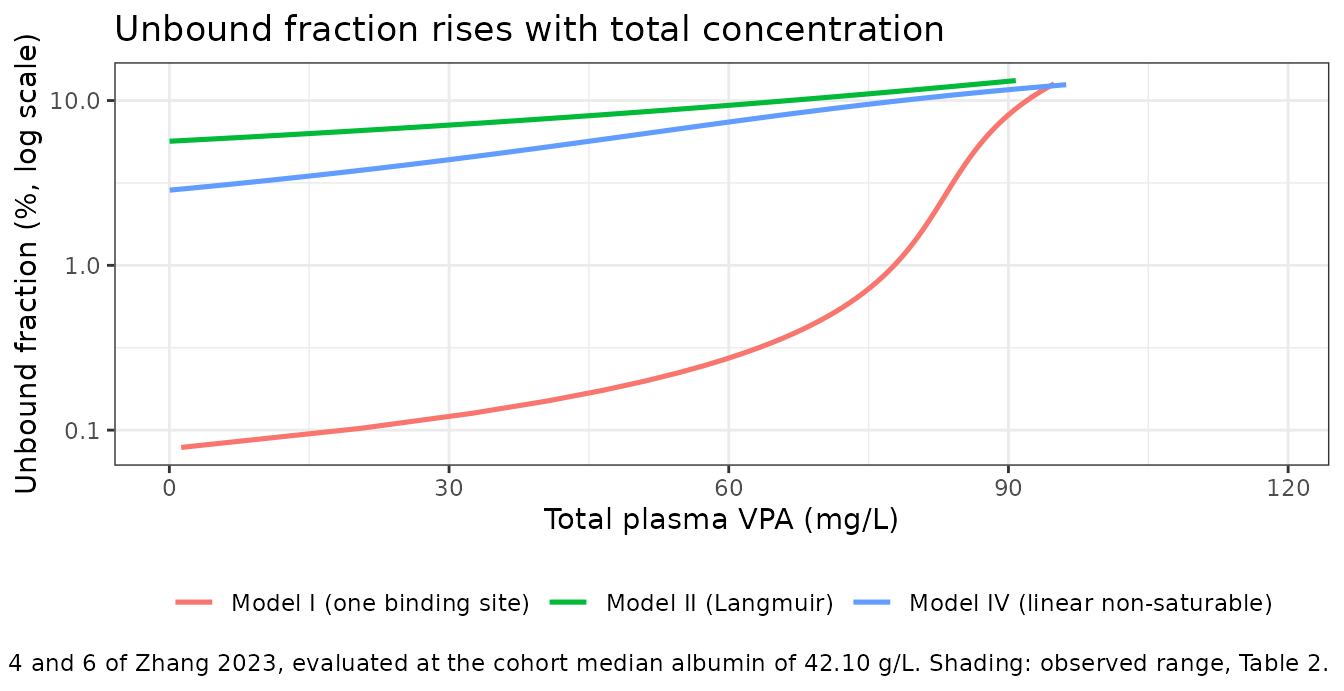

The three strategies disagree by orders of magnitude on the level of the unbound fraction while agreeing on the direction. Models II and IV put it near 8-10% over the observed range, consistent with the 90-95% protein binding the paper’s own Introduction quotes; Model I puts it near 0.3%, some thirty-fold lower. This is exactly the point the authors make in the Discussion: the one-binding-site constants were derived in adults, and age is positively correlated with the valproate free fraction, so that strategy transfers poorly to children. The level is absorbed into the unbound-referenced CLp/F, which is why Model I still predicts total concentrations in the right range.

Supplementary Figure S5B – clearance versus daily dose under Model V

Supplementary Figure S5B plots empirical Bayes estimates of VPA apparent clearance against daily dose for the simple exponent model, with the model-predicted typical clearance as a dashed line. The panel below reproduces that structure from the packaged model. As in the paper, the x-axis is the absolute daily dose in mg/day, so the curve reflects the joint distribution of weight and mg/kg dose in the cohort rather than being a pure function of the axis.

ebe <- sim |>
  filter(model == "Model V (simple exponent)") |>
  group_by(id, arm, WT, DOSE_VPA_MGKGD, DOSE_VPA_MGD) |>
  summarise(cl = first(cl), .groups = "drop")

typ_curve <- tibble(dd_mgkgd = seq(8.7, 57.7, length.out = 200)) |>
  mutate(cl = 0.331 * (dd_mgkgd / 25)^k_pub,
         DOSE_VPA_MGD = dd_mgkgd * 19)

ggplot(ebe, aes(DOSE_VPA_MGD, cl)) +
  geom_point(shape = 1, colour = "steelblue", alpha = 0.6) +
  geom_line(data = typ_curve, linetype = "dashed", colour = "red", linewidth = 0.9) +
  labs(x = "Daily dose (mg/d)", y = "Apparent clearance (L/h)",
       title = "The simple exponent model",
       caption = paste("Replicates Supplementary Figure S5B of Zhang 2023.",
                       "Dashed line: typical CL/F at the cohort median 19 kg.")) +
  theme_bw()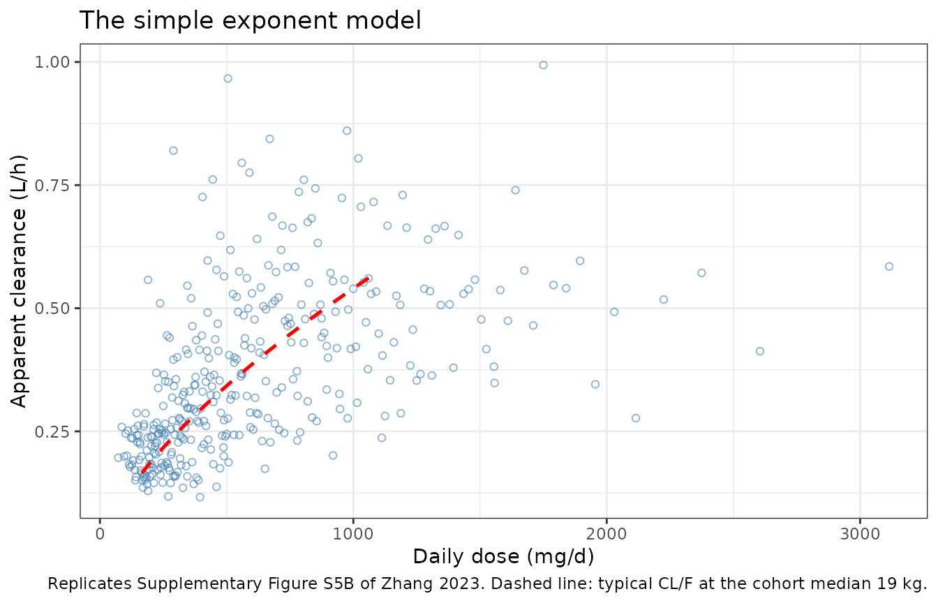

Supplementary Figure S5A – clearance versus daily dose under Model III

The same panel for the dose-dependent maximum effect model. This is the one figure the packaged Model III does not reproduce, and the discrepancy is recorded rather than tuned away: on the operator-ratified mg/day reading of DD50 the Hill term is nearly saturated across the whole observed dose range, so the typical curve is almost flat near 0.307 L/h, whereas the published Figure S5A rises from roughly 0.07 to 0.19 L/h. The Errata section sets out the conflicting evidence in full.

ebe3 <- sim |>
  filter(model == "Model III (dose-dependent Emax)") |>
  group_by(id, arm, DOSE_VPA_MGD) |>
  summarise(cl = first(cl), .groups = "drop")

typ3 <- tibble(DOSE_VPA_MGD = seq(60, 1250, length.out = 300)) |>
  mutate(cl = 0.0815 * (1 + 2.8 * DOSE_VPA_MGD^1.68 /
                          (37.4^1.68 + DOSE_VPA_MGD^1.68)))

ggplot(ebe3, aes(DOSE_VPA_MGD, cl)) +
  geom_point(shape = 1, colour = "steelblue", alpha = 0.6) +
  geom_line(data = typ3, linetype = "dashed", colour = "red", linewidth = 0.9) +
  labs(x = "Daily dose (mg/d)", y = "Apparent clearance (L/h)",
       title = "Dose-dependent maximum effect model",
       caption = paste("Structure of Supplementary Figure S5A of Zhang 2023.",
                       "The near-flat typical curve does NOT match the published",
                       "panel -- see Errata.")) +
  theme_bw()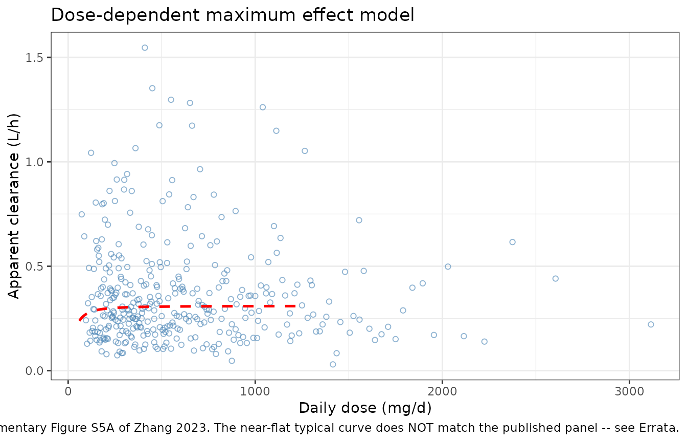

Steady-state concentration-time profiles

sim |>
  group_by(model, arm, time) |>
  summarise(Q05 = quantile(Cc, 0.05, na.rm = TRUE),
            Q50 = quantile(Cc, 0.50, na.rm = TRUE),
            Q95 = quantile(Cc, 0.95, na.rm = TRUE),
            .groups = "drop") |>
  ggplot(aes(time, Q50, colour = arm, fill = arm)) +
  geom_ribbon(aes(ymin = Q05, ymax = Q95), alpha = 0.2, colour = NA) +
  geom_line(linewidth = 0.8) +
  facet_wrap(~model, ncol = 2, scales = "free_y") +
  labs(x = "Time within the dosing interval (h)",
       y = "Total plasma VPA (mg/L)",
       colour = "Daily dose", fill = "Daily dose",
       title = "Steady-state profiles over one 12 h interval",
       caption = paste("Median with 5th-95th percentile band,", n_per_arm,
                       "subjects per arm. Note the compressed spacing of the",
                       "arms under every non-linear model.")) +
  theme_bw() +
  theme(legend.position = "bottom")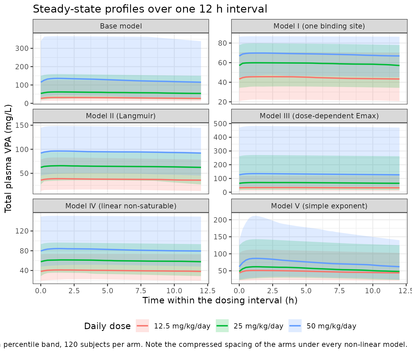

PKNCA validation

The paper’s own observations are steady-state troughs, so the NCA below is run over one complete 12 h steady-state dosing interval (Recipe 3). Because ss = 1 puts the system at steady state from time = 0, the time = 0 record is the steady-state trough and is a genuine measurement – the usual Cc = 0 pre-dose back-fill would be wrong here and is deliberately omitted.

sim_nca <- sim |>
  filter(!is.na(Cc)) |>
  select(model, id, time, Cc, arm)

# time = 0 is present by construction (it is the steady-state trough).
stopifnot(all(
  sim_nca |> group_by(model, id) |> summarise(has0 = any(time == 0), .groups = "drop") |> pull(has0)
))

dose_df <- events |>
  filter(evid == 1) |>
  select(id, time, amt, arm)

intervals <- data.frame(
  start = 0, end = tau,
  cmax = TRUE, tmax = TRUE, cmin = TRUE,
  auclast = TRUE, cav = TRUE
)

run_nca <- function(model_name) {
  conc_obj <- PKNCA::PKNCAconc(
    sim_nca |> filter(model == model_name) |> select(id, time, Cc, arm),
    Cc ~ time | arm + id, concu = "mg/L", timeu = "h"
  )
  dose_obj <- PKNCA::PKNCAdose(dose_df, amt ~ time | arm + id, doseu = "mg")
  PKNCA::pk.nca(PKNCA::PKNCAdata(conc_obj, dose_obj, intervals = intervals))
}

nca <- lapply(setNames(nm = names(model_names)), run_nca)

tidy_nca <- function(res, model_name) {
  as.data.frame(res$result) |>
    # PKNCA emits dependency rows; filter on the interval as well as the code
    filter(start == 0, end == tau,
           PPTESTCD %in% c("cmax", "tmax", "cmin", "auclast", "cav")) |>
    group_by(arm, PPTESTCD) |>
    summarise(median = median(PPORRES, na.rm = TRUE), .groups = "drop") |>
    mutate(model = model_name)
}

nca_tbl <- bind_rows(lapply(names(nca), \(m) tidy_nca(nca[[m]], m)))

nca_tbl |>
  mutate(median = round(median, 2),
         Parameter = nlmixr2lib::ncaParamLabel(PPTESTCD)) |>
  select(model, arm, Parameter, median) |>
  tidyr::pivot_wider(names_from = Parameter, values_from = median) |>
  rename("Model" = model, "Arm" = arm) |>
  knitr::kable(caption = paste("Median steady-state NCA over one 12 h interval.",
                               "Cmin is the trough the paper's TDM samples measured."))

Median steady-state NCA over one 12 h interval. Cmin is the trough the paper’s TDM samples measured.
Model	Arm	AUClast	Cavg	Cmax	Cmin	Tmax
Base model	12.5 mg/kg/day	362.55	30.21	31.93	26.72	1.25
Base model	25 mg/kg/day	696.61	58.05	61.86	53.88	1.25
Base model	50 mg/kg/day	1504.50	125.37	135.98	115.06	1.25
Model I (one binding site)	12.5 mg/kg/day	534.23	44.52	45.77	43.31	1.25
Model I (one binding site)	25 mg/kg/day	710.07	59.17	59.85	57.06	1.25
Model I (one binding site)	50 mg/kg/day	824.08	68.67	69.81	66.84	1.25
Model II (Langmuir)	12.5 mg/kg/day	449.56	37.46	38.78	35.72	1.25
Model II (Langmuir)	25 mg/kg/day	770.99	64.25	66.01	62.30	1.25
Model II (Langmuir)	50 mg/kg/day	1132.41	94.37	96.31	92.04	1.25
Model III (dose-dependent Emax)	12.5 mg/kg/day	395.49	32.96	33.83	31.99	1.25
Model III (dose-dependent Emax)	25 mg/kg/day	819.45	68.29	70.46	64.77	1.25
Model III (dose-dependent Emax)	50 mg/kg/day	1572.69	131.06	135.06	126.41	1.25
Model IV (linear non-saturable)	12.5 mg/kg/day	477.33	39.78	41.21	38.12	1.25
Model IV (linear non-saturable)	25 mg/kg/day	714.47	59.54	61.50	57.81	1.25
Model IV (linear non-saturable)	50 mg/kg/day	980.50	81.71	84.43	79.44	1.25
Model V (simple exponent)	12.5 mg/kg/day	572.10	47.67	51.07	44.11	1.25
Model V (simple exponent)	25 mg/kg/day	668.40	55.70	62.02	48.15	1.25
Model V (simple exponent)	50 mg/kg/day	878.03	73.17	86.50	62.16	1.25

Comparison against the published concentration

Zhang et al. report no NCA table – their cohort is trough-only TDM data, and their model metrics are prediction errors against individual observations that are not public. The one published concentration that a simulation can be held against is the observed steady-state trough itself: median 50.40 mg/L (mean 54.34, range 22.60-118.50; Table 2), at a cohort median daily dose of 23.44 mg/kg/day. The 25 mg/kg/day arm is the closest match.

published <- tibble::tribble(
  ~arm,             ~cmin,
  "25 mg/kg/day",   50.40
)

cmp <- bind_rows(lapply(names(nca), function(m) {
  nlmixr2lib::ncaComparisonTable(
    simulated = nca[[m]], reference = published, by = "arm",
    units = c(cmin = "mg/L"), tolerance_pct = 20
  ) |>
    mutate(Model = m)
})) |>
  relocate(Model)

cmp |>
  knitr::kable(
    caption = paste("Simulated vs published steady-state trough (Zhang 2023 Table 2).",
                    "* differs from the reference by more than 20%."),
    align = c("l", "l", "l", "r", "r", "r")
  )

Simulated vs published steady-state trough (Zhang 2023 Table 2). * differs from the reference by more than 20%.
Model	NCA parameter	arm	Reference	Simulated	% diff
Base model	Cmin (mg/L)	25 mg/kg/day	50.4	53.9	+6.9%
Model I (one binding site)	Cmin (mg/L)	25 mg/kg/day	50.4	57.1	+13.2%
Model II (Langmuir)	Cmin (mg/L)	25 mg/kg/day	50.4	62.3	+23.6%*
Model III (dose-dependent Emax)	Cmin (mg/L)	25 mg/kg/day	50.4	64.8	+28.5%*
Model IV (linear non-saturable)	Cmin (mg/L)	25 mg/kg/day	50.4	57.8	+14.7%
Model V (simple exponent)	Cmin (mg/L)	25 mg/kg/day	50.4	48.2	-4.5%

The coherence of the family is the real result here, not the individual percentages. The six models were fit to the same 255 observations, so their predictions must land together – and they do: every simulated trough falls between about 48 and 65 mg/L, a spread of well under two-fold, even though the six published CLp/F values span more than three orders of magnitude (0.0815 to 132 L/h). That is what confirms Models I, II and IV are unbound-referenced. A total-concentration reading of their CLp/F would put their predictions one to three orders of magnitude out, not tens of per cent. The same coherence is what the operator’s ratified DD50 reading for Model III was chosen to preserve.

Two rows star at the 20% tolerance (Models II and III), and the family as a whole sits above the published 50.40 mg/L rather than centred on it. Read that as a property of the comparison rather than of the transcription. The published figure is a marginal median over a cohort spanning 8.70-57.69 mg/kg/day given one to three times daily; the arm here is a single fixed 25 mg/kg/day given twice daily, above the cohort’s median 23.44 mg/kg/day. None of these models scales CL/F by weight, so the simulated trough is proportional to body weight while the dose per kilogram is held fixed – a mismatch a marginal median cannot be corrected for without the individual records, which are not public. What tests the encoding is the set of exact identities in the structural-checks section above, all of which hold to numerical precision; the paper’s own near-zero MDPEs are computed against those individual observations and are not reproducible here. No parameter was tuned and no tolerance was widened to unstar a row.

Two further caveats on what this check does and does not establish. It compares medians across variable populations, so it validates the central tendency of CL/F and the steady-state trough machinery, but says nothing about the variance structure – and the paper is explicit that variance was where every model it evaluated performed badly (all models were rejected by the normalised prediction distribution error global test). It also uses three fixed mg/kg/day strata in place of a cohort spanning 8.70-57.69 mg/kg/day and one to three doses daily, so it cannot detect a misspecified dose-dependence; the exact identities in the structural-checks section above are what pin that.

Assumptions and deviations

Cohort composition is reconstructed, not published. Weights are placed on lognormal quantiles with the median pinned to the published 19.00 kg and clamped to the published 4.00-70.00 kg range; albumin on normal quantiles with the median pinned to 42.10 g/L and clamped to 29.70-70.50 g/L. The paper reports only summary statistics (Table 2), not the joint distribution of weight, age, albumin and dose. Deterministic quantiles are used in preference to a random draw so the cohort medians match the published values exactly and the vignette is seed-independent. The sustained-release fraction is set to 61/255 to match the record counts in Table 2. Age is not simulated at all, because no model in this paper uses it.
Twice-daily dosing was chosen for the simulation. The paper states dosing was “one, two, or three times per day” without reporting the mix, so a single representative interval (tau = 12 h) is used throughout.
Steady state is imposed with ss = 1. The apparent terminal half-life implied by the published parameters runs from about 36 h (Model V) to about 120 h (Model III), so dosing up from zero would not reach the trough the paper observed within a tractable simulation horizon.
V/F is large relative to the paediatric VPA literature (27.8 L for a cohort with a 19 kg median weight, about 1.5 L/kg, against a literature value near 0.2 L/kg). This is faithful to the source: the authors state that because their data were “mostly at trough concentrations … parameters for the absorption and distribution stages could not be obtained precisely.” The parameter is reproduced as published and not adjusted.
Models I, II and IV are carried on the unbound concentration. The paper prints Equations 3, 4 and 6 as bare Cb-versus-Cu isotherms and never says how they couple to the PK. The coupling used here – Cu = central / (V/F), elimination CL * Cu, observation Cc = Cu + Cb – is not a guess: it is confirmed three times over per model by the fu reconciliation table above, and it is the only reading under which the published CLp/F and V/F produce concentrations in the observed range.
Model I’s units are dimensionally inconsistent as printed. The paper gives K = 15.5 mM^-1 and N = 1.98. Evaluating Equation 3 with Cu and ALB converted to molar units gives a typical total concentration of 3.3 mg/L, 17-fold below the observed median of 50.4 mg/L. Evaluating it with Cu in mg/L, ALB in g/L and K at its printed numeric value gives 59.9 mg/L and reproduces the 0.24% / 0.21% unbound fraction implied independently by the CL/F and V/F ratios. The numerically-consistent reading is implemented and the printed mM^-1 label is treated as an error.
DD in Equation 7 is implemented on the mg/kg/day scale. The paper’s abbreviation list defines DD as daily dose in mg/day and DDW as daily dose in mg/kg/day, and Equation 7 is printed with DD. However the equation reads (DD/25), and 25 matches the cohort mean daily dose of 24.50 mg/kg/day (Table 2), not any mg/day quantity; and the reported CLp/F of 0.331 L/h reproduces the base-model CL/F of 0.311 L/h only on the mg/kg/day reading. On the mg/day reading, typical clearance comes out at 2.42 L/h and the predicted trough at about 9 mg/L, against an observed median of 50.40 mg/L. The mg/kg/day reading is therefore used, and the text’s DD/DDW label is treated as a typographical inconsistency. This is recorded in the DOSE_VPA_MGKGD register entry.
No covariates on CL/F or V/F. None of the six models carries a weight, age or co-medication effect, and albumin appears only inside Model I’s isotherm. This is unusual for a paediatric model and is faithful to Supplementary Table S3; weight is recorded in covariatesDataExcluded in every model file with the reason.
Models III and V are not dosing tools. The authors argue explicitly that because the daily dose is the quantity a TDM model exists to predict, using it as a clearance covariate is circular. They conclude the simple exponent form “did not describe the non-linear properties of the VPA PK process” despite its good prediction metrics, and Model III was the worst performer of the five. Both are packaged for fidelity to the published comparison.
Between-subject variability is diagonal. Zhang 2023 reports no CL/F-V/F correlation for its own models, so no off-diagonal is encoded.
Non-paper-derived values: one. Every ini() value comes from the paper’s Equations 3-7 or Supplementary Table S3, except Model III’s DD50 (next item). The Ka shift parameters are log-ratios computed from the three published fixed Ka values (2.64 / 1.57 / 0.46 1/h); the arithmetic is visible in each model file.

Errata: Model III’s unreported `DD50`

Equation 5 needs Emax, a Hill coefficient and DD50. The paper fixes Emax = 2.8 and the Hill coefficient at 1.68 “as reported (Ding et al., 2015)” but never reports DD50 – it is absent from Supplementary Table S3 (whose CL_DD row is “/” for this model) and from the body text. The value used here, DD50 = 37.4, is Ding 2015’s own value, tabulated in Zhang’s own Table 1, read on the mg/day scale. This is an operator-ratified decision (sidecar oare_PMC10587682, question 2, option C), not a value the paper states.

The evidence conflicts, and the conflict is genuine:

For the mg/day reading (implemented). Typical CL/F comes out at 0.307 L/h against the base model’s 0.311 L/h, and the typical steady-state concentration lands with the other five models rather than 2.7-fold above them. Table 3 reports an MDPE of -1.10% for this model, which is only reachable if its typical predictions sit near the observed median.
For the mg/kg/day reading (not implemented). Equation 5’s own text defines DD50 as “the daily dose (mg kg-1 day-1)”, and Ding 2015 tabulates 37.4 against a per-kilogram daily dose. Supplementary Figure S5A supports it too: digitising the published typical curve at the cohort median daily dose of 480 mg/day gives a typical CL/F near 0.152 L/h, which back-solves to DD50 = 37.9 mg/kg/day – within 1.3% of Ding’s 37.4 on the per-kilogram scale.

So Supplementary Figure S5A and Table 3 are in tension with each other for this model independently of which scale is chosen: S5A shows a typical CL/F around half the base model’s, which would necessarily produce a large positive prediction error, not the near-zero one reported. A further diagnostic points the same way: Model III’s objective function value (1773.0) is worse than the base model’s (1752.1), and since the base model is the DD50 -> infinity limiting case of Equation 5 with CLp/F free, an estimated DD50 could not have raised the OFV – so DD50 was fixed, not estimated.

The ratified choice preserves the reported predictive performance at the cost of the reported figure. A user who wants the other reading only needs to divide DOSE_VPA_MGD by body weight before passing it in; nothing else changes. The Zhang_2023_valproic_acid_ddemax model file carries the same note at the dd_50 parameter.