Loperamide and N-desmethyl loperamide concentration-QTc (Valenzuela 2025)
Source:vignettes/articles/Valenzuela_2025_loperamide.Rmd
Valenzuela_2025_loperamide.RmdModel and source
Valenzuela 2025 analysed a four-way crossover thorough-QT study of single oral loperamide doses (8 mg therapeutic, 48 mg supratherapeutic) with placebo and moxifloxacin controls. The paper reports two fit-for-purpose population PK models (loperamide, and its N-desmethyl metabolite M1 treated as if dosed independently) and two concentration-QTc models that differ only in the analyte driving the effect compartment. The package therefore ships two model files, each a PK model with its own effect compartment and linear concentration-ddQTcF model:
Valenzuela_2025_loperamide_QTcF_M1– the primary model, driven by M1.Valenzuela_2025_loperamide_QTcF_parent– the sensitivity-analysis model, driven by loperamide.Citation: Valenzuela B, Gisleskog PO, Cirillo I, Coenen E, Ariyawansa J, Ali SR, Takhtoukh S, Perez-Ruixo JJ, Ackaert O. Evaluation of the Effect of Loperamide on the Cardiac Repolarization Interval Using Exposure-Response Analysis. Clin Transl Sci. 2025;18(2):e70114. doi:10.1111/cts.70114.
Description (M1): Population PK / concentration-QTc model for N-desmethyl loperamide (M1), the major metabolite of loperamide, in healthy adults from a randomized, placebo- and moxifloxacin-controlled four-way crossover thorough-QT study (NCT04225078; single oral loperamide 8 mg and 48 mg). This is the paper’s primary exposure-response model. Fit-for-purpose M1 PK with the metabolite treated as if dosed independently: the loperamide dose enters a depot by a zero-order input after a lag time and reaches a two-compartment M1 disposition model by first-order absorption; the 48 mg dose has its own relative bioavailability, absorption rate constant and lag time. IIV on Vc/F, F and ka; inter-occasion variability on the lag time and the zero-order duration. An effect compartment (ke0) on the M1 concentration drives the prespecified linear model for the placebo-adjusted change from baseline in Fridericia-corrected QT (ddQTcF = (b0 + eta) + (b1 + eta) * Ce + b2 * (QTcF baseline - mean)). The loperamide-driven sensitivity model is Valenzuela_2025_loperamide_QTcF_parent.
Description (parent): Population PK / concentration-QTc model for loperamide (parent) in healthy adults from a randomized, placebo- and moxifloxacin-controlled four-way crossover thorough-QT study (NCT04225078; single oral loperamide 8 mg and 48 mg). Fit-for-purpose PK: two-compartment disposition with linear elimination and sequential zero- then first-order absorption after a lag time; the 48 mg dose has its own relative bioavailability, absorption rate constant and lag time. IIV on Vc/F, F and ka; inter-occasion variability on the lag time and the zero-order duration. An effect compartment (ke0) drives the prespecified linear model for the placebo-adjusted change from baseline in Fridericia-corrected QT (ddQTcF = (b0 + eta) + (b1 + eta) * Ce + b2 * (QTcF baseline - mean)). This loperamide-driven exposure-response model is the paper’s sensitivity analysis; the primary model is driven by the N-desmethyl metabolite M1 (Valenzuela_2025_loperamide_QTcF_M1).
Article: https://doi.org/10.1111/cts.70114 (open access; PMC11770325)
Population
The study (NCT04225078) enrolled 65 healthy adults (22 male, 43 female) aged 18-55 years with a body mass index of 18-30 kg/m^2 and body weight of at least 50 kg, at a single centre in Belgium between January 2020 and January 2022. Participants received single oral doses of loperamide 8 mg, loperamide 48 mg, moxifloxacin 400 mg and placebo in four periods separated by washouts of at least 7 days. ECGs were extracted in triplicate from continuous 12-lead Holter recordings at 0.5 to 36 h after dosing, time-matched to the PK samples. The exposure-response dataset holds 1408 time-matched PK and ddQTcF records from 53 participants (51 at 8 mg, 50 at 48 mg). The paper reports no table of baseline demographics beyond these figures (Methods and Results, Dataset).
The same information is available programmatically:
str(readModelDb("Valenzuela_2025_loperamide_QTcF_M1")()$population)
#> Warning: some etas defaulted to non-mu referenced, possible parsing error: etaiov_ltlag_1, etaiov_ltlag_2, etaiov_ld1_1, etaiov_ld1_2, etaslope
#> as a work-around try putting the mu-referenced expression on a simple line
#> List of 11
#>  $ species       : chr "human"
#>  $ n_subjects    : int 53
#>  $ n_studies     : int 1
#>  $ n_observations: int 1408
#>  $ age_range     : chr "18-55 years (eligibility criterion; observed range not reported)"
#>  $ weight_range  : chr ">= 50 kg; BMI 18-30 kg/m^2 (eligibility criteria)"
#>  $ sex_female_pct: num 66.2
#>  $ disease_state : chr "Healthy adult volunteers"
#>  $ dose_range    : chr "Single oral loperamide 8 mg (therapeutic; 51 participants) and 48 mg (supratherapeutic; 50 participants), place"| __truncated__
#>  $ regions       : chr "Belgium"
#>  $ notes         : chr "Thorough-QT study NCT04225078, conducted January 2020 to January 2022. 65 participants were enrolled (22 male, "| __truncated__
Source trace
Every ini() value carries an in-file comment pointing to
its table row. Both PK models share the same structure (Valenzuela 2025
Figure S3) and both exposure-response models share Equation 1.
| Equation / parameter | Loperamide | M1 | Source location |
|---|---|---|---|
lcl / lcl_m1 (CL/F, L/h) |
293 | 52.4 | Table 1 |
lvc / lvc_m1 (Vc/F, L) |
3380 | 1650 | Table 1 |
lvp / lvp_m1 (Vp/F, L) |
1770 | 805 | Table 1 |
lq / lq_m1 (Q/F, L/h) |
219 | 96.4 | Table 1 |
lfdepot (F, 8 mg) |
1 fixed | 1 fixed | Table 1 |
lfdepot_highdose (F, 48 mg) |
1.20 | 1.10 | Table 1 |
lka (ka, 8 mg, 1/h) |
1.19 | 0.258 | Table 1 |
lka_highdose (ka, 48 mg, 1/h) |
4.21 | 0.991 | Table 1 |
ltlag (lag, 8 mg, h) |
0.149 | 0.162 | Table 1 |
ltlag_highdose (lag, 48 mg, h) |
0.271 | 0.376 | Table 1 |
ld1 (zero-order duration D1, h) |
0.551 | 0.714 | Table 1 |
| IIV Vc/F, F, ka (%CV) | 19.6, 43.5, 98.6 | 32.3, 20.8, 40.6 | Table 1 |
| IOV lag, D1 (%CV) | 76.2, 72.9 | 59.3, 97.1 | Table 1, footnote a |
propSd / propSd_m1
|
0.177 | 0.171 | Table 1, footnote b (additive on log scale) |
lke0 (1/h) |
0.024 | 0.094 | Table 2 |
e0 intercept (ms) |
-1.76 | -1.66 | Table 2 |
slope (ms per ng/mL) |
2.91 | 0.544 | Table 2 |
e_qtc_bl_e0 (ms per ms) |
-0.173 | -0.155 | Table 2 |
etae0, etaslope, etalke0
(variances) |
17.7, 0.00001, 0.947 | 15.7, 0.143, 0.748 | Table 2 |
addSd (ms) |
sqrt(42.8) | sqrt(41.7) | Table 2 |
| Sequential zero- then first-order absorption after a lag | Results; Figure S3 | ||
d/dt(effect) = ke0 * (C - effect) |
Methods (effect compartment, ref. 14); Figure S3 | ||
QTcF = (e0 + eta) + (slope + eta) * Ce + e_qtc_bl_e0 * (QTC_BL - 400) |
Equation 1 |
Typical-value check against the reported ddQTcF
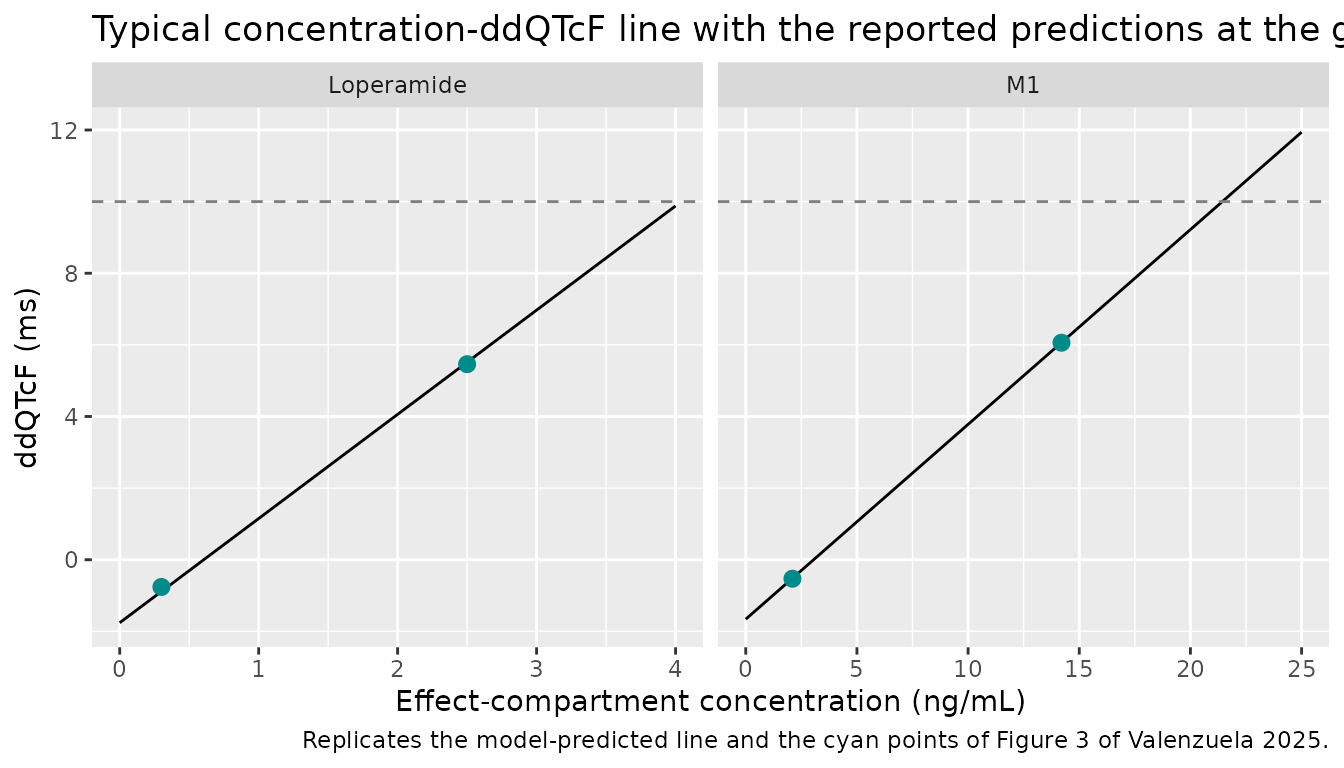
The paper reports the model-predicted mean ddQTcF at the predicted
geometric mean effect-compartment Cmax of each dose (Results; Figure 3).
Equation 2 of the paper is the typical linear prediction
b0 + Cmax * b1, so the packaged intercept and slope must
reproduce those numbers at the printed concentrations. This is a check
on the transcription of the intercept and slope, independent of any
simulation.
theta_of <- function(name) {
  ui <- rxode2::rxode(readModelDb(name))
  ui$theta
}
th_m1 <- theta_of("Valenzuela_2025_loperamide_QTcF_M1")
#> ℹ parameter labels from comments will be replaced by 'label()'
#> Warning: some etas defaulted to non-mu referenced, possible parsing error: etaiov_ltlag_1, etaiov_ltlag_2, etaiov_ld1_1, etaiov_ld1_2, etaslope
#> as a work-around try putting the mu-referenced expression on a simple line
th_p <- theta_of("Valenzuela_2025_loperamide_QTcF_parent")
#> ℹ parameter labels from comments will be replaced by 'label()'
#> Warning: some etas defaulted to non-mu referenced, possible parsing error: etaiov_ltlag_1, etaiov_ltlag_2, etaiov_ld1_1, etaiov_ld1_2, etaslope
#> as a work-around try putting the mu-referenced expression on a simple line

reported <- tibble::tribble(
  ~model, ~dose, ~ce_gm, ~ddqtcf_reported,
  "M1", "8 mg", 2.1, -0.53,
  "M1", "48 mg", 14.2, 6.06,
  "Loperamide", "8 mg", 0.3, -0.76,
  "Loperamide", "48 mg", 2.5, 5.46
)
typical <- reported |>
  mutate(
    ddqtcf_model = ifelse(
      model == "M1",
      th_m1[["e0"]] + th_m1[["slope"]] * ce_gm,
      th_p[["e0"]] + th_p[["slope"]] * ce_gm
    ),
    difference = ddqtcf_model - ddqtcf_reported
  )

typical |>
  rename(
    "Model" = model, "Dose" = dose,
    "Geometric mean Ce,max (ng/mL)" = ce_gm,
    "Reported ddQTcF (ms)" = ddqtcf_reported,
    "Packaged model ddQTcF (ms)" = ddqtcf_model,
    "Difference (ms)" = difference
  ) |>
knitr::kable(digits = 3, caption = "Typical ddQTcF at the reported geometric-mean effect-compartment Cmax.")| Model | Dose | Geometric mean Ce,max (ng/mL) | Reported ddQTcF (ms) | Packaged model ddQTcF (ms) | Difference (ms) |
|---|---|---|---|---|---|
| M1 | 8 mg | 2.1 | -0.53 | -0.518 | 0.012 |
| M1 | 48 mg | 14.2 | 6.06 | 6.065 | 0.005 |
| Loperamide | 8 mg | 0.3 | -0.76 | -0.887 | -0.127 |
| Loperamide | 48 mg | 2.5 | 5.46 | 5.515 | 0.055 |
Virtual cohort
Observed data are not public. Each model is simulated in a virtual cohort of 150 participants per dose, treated as parallel arms (the crossover’s within-participant pairing does not change the per-dose distributions). The 8 mg arm is occasion 1 and the 48 mg arm occasion 2, so each draws its own inter-occasion random effects. Every participant’s baseline QTcF is set to the 400 ms centering value, because the paper reports neither the mean nor the spread of baseline QTcF.
n_per_arm <- 150L
obs_times <- sort(unique(c(seq(0, 2, by = 0.125), seq(2.5, 12, by = 0.5), seq(13, 36, by = 1))))

make_arm <- function(n, dose_mg, id_offset) {
  ids <- id_offset + seq_len(n)
  high <- as.integer(dose_mg == 48)
  covs <- data.frame(id = ids, DOSE_HIGH = high, OCC = ifelse(high == 1L, 2L, 1L), QTC_BL = 400)
  # The models have two error endpoints, neither of which is an ODE state, so
  # observation rows nominate the first endpoint through dvid; rxSolve still
  # returns every endpoint as a column. Zero-order input: rate = -2 lets the
  # model's dur(depot) set the duration.
  dose_rows <- data.frame(
    id = ids, time = 0, amt = dose_mg, evid = 1L, cmt = "depot",
    rate = -2, dvid = NA_integer_
  )
  obs_rows <- expand.grid(id = ids, time = obs_times) |>
    mutate(amt = 0, evid = 0L, cmt = NA_character_, rate = 0, dvid = 1L)
  bind_rows(dose_rows, obs_rows) |>
    left_join(covs, by = "id") |>
    mutate(dose = paste(dose_mg, "mg")) |>
    arrange(id, time, desc(evid))
}

events <- bind_rows(
  make_arm(n_per_arm, 8, id_offset = 0L),
  make_arm(n_per_arm, 48, id_offset = n_per_arm)
)
stopifnot(!anyDuplicated(unique(events[, c("id", "time", "evid")])))
Simulation
mod_m1 <- readModelDb("Valenzuela_2025_loperamide_QTcF_M1")
mod_p <- readModelDb("Valenzuela_2025_loperamide_QTcF_parent")

rxode2::rxSetSeed(2025)
sim_m1 <- rxode2::rxSolve(mod_m1, events = events, keep = c("dose")) |>
  as.data.frame()
#> ℹ parameter labels from comments will be replaced by 'label()'
#> Warning: some etas defaulted to non-mu referenced, possible parsing error: etaiov_ltlag_1, etaiov_ltlag_2, etaiov_ld1_1, etaiov_ld1_2, etaslope
#> as a work-around try putting the mu-referenced expression on a simple line
rxode2::rxSetSeed(2026)
sim_p <- rxode2::rxSolve(mod_p, events = events, keep = c("dose")) |>
  as.data.frame()
#> ℹ parameter labels from comments will be replaced by 'label()'
#> Warning: some etas defaulted to non-mu referenced, possible parsing error: etaiov_ltlag_1, etaiov_ltlag_2, etaiov_ld1_1, etaiov_ld1_2, etaslope
#> as a work-around try putting the mu-referenced expression on a simple line

stopifnot(
  !anyNA(sim_m1$Cc_m1), !anyNA(sim_m1$QTcF),
  !anyNA(sim_p$Cc), !anyNA(sim_p$QTcF)
)
The in-model Cc, Cc_m1 and
QTcF columns are individual predictions (no residual
error). The VPC below adds the published residual error so that it is
comparable to the paper’s observation-based percentiles.
Replicate Figure 1 (PK visual predictive check)
vpc_pk <- bind_rows(
  sim_p |> transmute(id, time, dose, analyte = "Loperamide", ipred = Cc,
                     sd = rxode2::rxode(mod_p)$theta[["propSd"]]),
  sim_m1 |> transmute(id, time, dose, analyte = "M1", ipred = Cc_m1,
                      sd = rxode2::rxode(mod_m1)$theta[["propSd_m1"]])
) |>
  filter(time %in% obs_times[-1]) |> # drop the pre-dose zero for the log axis
  mutate(dv = ipred * exp(rnorm(n(), 0, sd))) |>
  group_by(analyte, dose, time) |>
  summarise(
    p10 = quantile(dv, 0.10), p50 = quantile(dv, 0.50), p90 = quantile(dv, 0.90),
    .groups = "drop"
  ) |>
  mutate(dose = factor(dose, levels = c("8 mg", "48 mg")))
#> ℹ parameter labels from comments will be replaced by 'label()'
#> Warning: There was 1 warning in `transmute()`.
#> ℹ In argument: `sd = rxode2::rxode(mod_p)$theta[["propSd"]]`.
#> Caused by warning:
#> ! some etas defaulted to non-mu referenced, possible parsing error: etaiov_ltlag_1, etaiov_ltlag_2, etaiov_ld1_1, etaiov_ld1_2, etaslope
#> as a work-around try putting the mu-referenced expression on a simple line
#> ℹ parameter labels from comments will be replaced by 'label()'
#> Warning: There was 1 warning in `transmute()`.
#> ℹ In argument: `sd = rxode2::rxode(mod_m1)$theta[["propSd_m1"]]`.
#> Caused by warning:
#> ! some etas defaulted to non-mu referenced, possible parsing error: etaiov_ltlag_1, etaiov_ltlag_2, etaiov_ld1_1, etaiov_ld1_2, etaslope
#> as a work-around try putting the mu-referenced expression on a simple line

ggplot(vpc_pk, aes(time, p50)) +
  geom_ribbon(aes(ymin = p10, ymax = p90), fill = "steelblue", alpha = 0.3) +
  geom_line() +
  facet_grid(analyte ~ dose, scales = "free_y") +
  scale_y_log10() +
  labs(
    x = "Time after dose (h)", y = "Plasma concentration (ng/mL)",
    title = "Simulated median and 80% prediction interval",
    caption = "Replicates Figure 1 of Valenzuela 2025 (VPC of loperamide and M1 PK)."
  )
#> Warning in scale_y_log10(): log-10 transformation introduced infinite values.
#> Warning in scale_y_log10(): log-10 transformation introduced infinite values.
#> log-10 transformation introduced infinite values.
#> log-10 transformation introduced infinite values.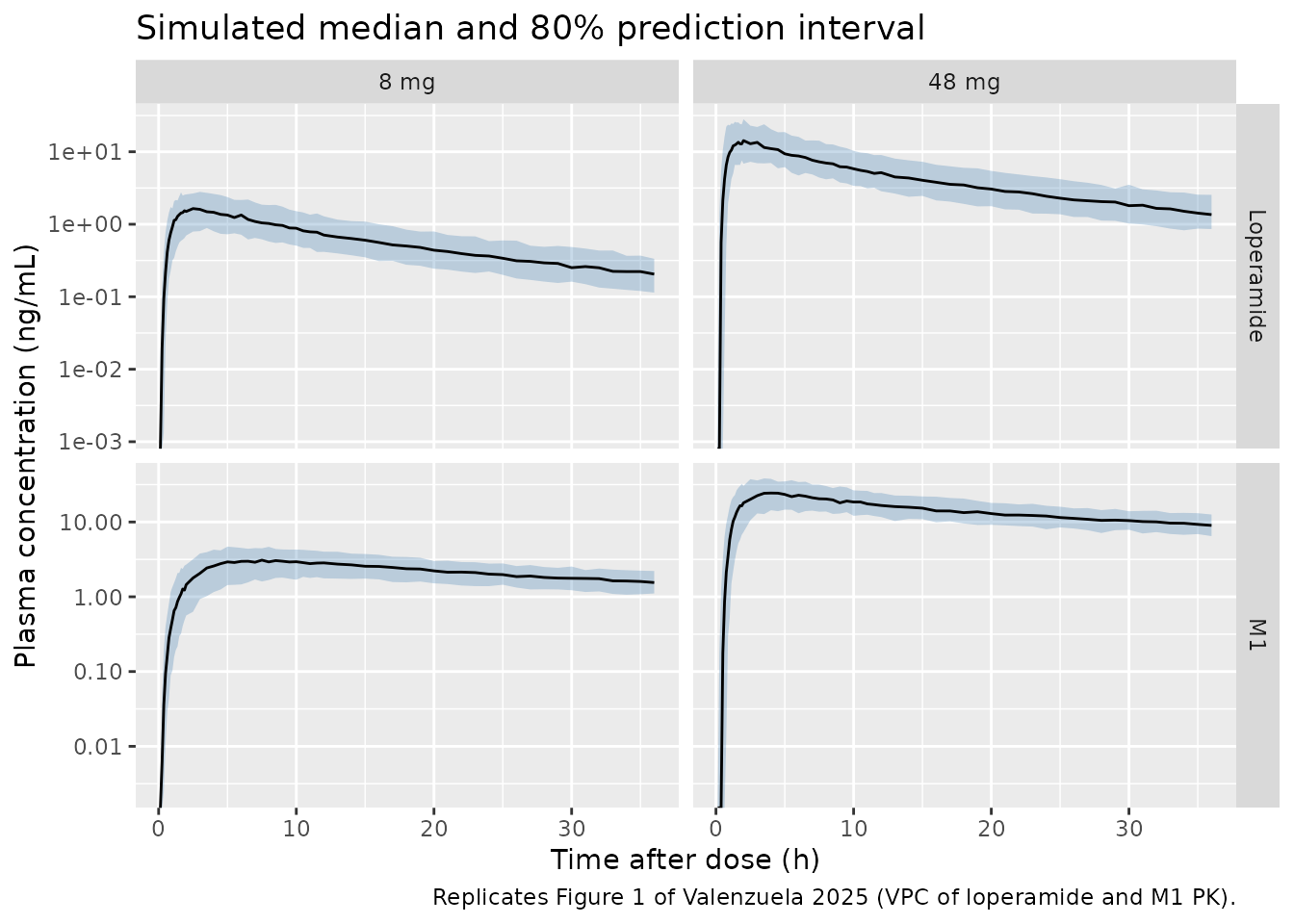
Effect-compartment Cmax and ddQTcF
The paper reports the predicted geometric-mean Cmax in the effect compartment per dose: 2.1 and 14.2 ng/mL for M1 and 0.3 and 2.5 ng/mL for loperamide after 8 and 48 mg (Results). The simulated cohort’s geometric means over the 0-36 h sampling window are compared below. The effect compartment of loperamide equilibrates slowly (1/ke0 = 42 h), so its peak falls late in that window.
ce_max <- bind_rows(
  sim_m1 |> mutate(model = "M1"),
  sim_p |> mutate(model = "Loperamide")
) |>
  group_by(model, dose, id) |>
  summarise(ce_max = max(effect), .groups = "drop") |>
  group_by(model, dose) |>
  summarise(gm_sim = exp(mean(log(ce_max))), .groups = "drop") |>
  inner_join(reported |> select(model, dose, ce_gm), by = c("model", "dose")) |>
  mutate(pct_diff = 100 * (gm_sim / ce_gm - 1))

ce_max |>
  rename(
    "Model" = model, "Dose" = dose,
    "Simulated geometric mean Ce,max (ng/mL)" = gm_sim,
    "Reported (ng/mL)" = ce_gm, "Difference (%)" = pct_diff
  ) |>
knitr::kable(digits = 2, caption = "Geometric-mean effect-compartment Cmax, simulated vs. reported.")| Model | Dose | Simulated geometric mean Ce,max (ng/mL) | Reported (ng/mL) | Difference (%) |
|---|---|---|---|---|
| Loperamide | 48 mg | 2.31 | 2.5 | -7.44 |
| Loperamide | 8 mg | 0.32 | 0.3 | 6.12 |
| M1 | 48 mg | 13.14 | 14.2 | -7.47 |
| M1 | 8 mg | 2.02 | 2.1 | -3.93 |
# The cohort geometric mean is a centre statistic (robust to which participants
# land in the tails); a mis-transcribed CL/F, volume, F or ke0 moves it by
# tens of percent. The 8 mg loperamide value (0.3 ng/mL) is printed to one
# significant figure, so it is held to the rounding interval 0.25-0.35 widened
# by the same margin.
stopifnot(all(abs(ce_max$pct_diff[!(ce_max$model == "Loperamide" & ce_max$dose == "8 mg")]) < 25))
stopifnot(abs(ce_max$pct_diff[ce_max$model == "Loperamide" & ce_max$dose == "8 mg"]) < 40)
dd_time <- bind_rows(
  sim_m1 |> mutate(model = "M1 model (primary)"),
  sim_p |> mutate(model = "Loperamide model (sensitivity)")
) |>
  group_by(model, dose, time) |>
  summarise(mean_ddqtcf = mean(QTcF), .groups = "drop") |>
  mutate(dose = factor(dose, levels = c("8 mg", "48 mg")))

ggplot(dd_time, aes(time, mean_ddqtcf, colour = dose)) +
  geom_line() +
  geom_hline(yintercept = 0, colour = "grey50") +
  geom_hline(yintercept = 10, linetype = "dashed", colour = "grey50") +
  facet_wrap(~model) +
  labs(
    x = "Time after dose (h)", y = "Mean ddQTcF (ms)", colour = "Dose",
    title = "Simulated mean ddQTcF over time",
    caption = "Compare with Figure S6 of Valenzuela 2025 (observed mean ddQTcF by time point)."
  )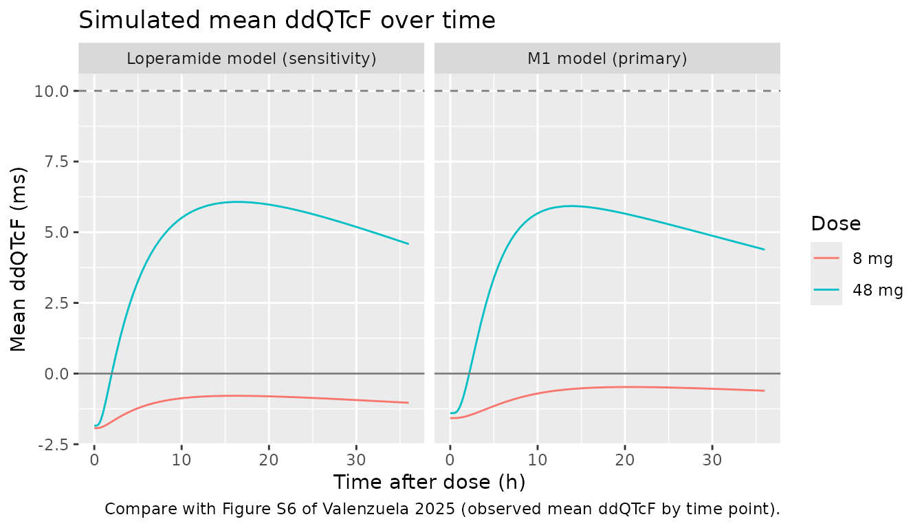
# Figure S6: after 48 mg the observed mean ddQTcF exceeded 5 ms at 8, 12 and
# 24 h; after 8 mg it stayed near zero. Assert the centre of the simulated
# 48 mg profile over 8-24 h sits well above the 8 mg one and below 10 ms.
m1_48 <- dd_time |> filter(model == "M1 model (primary)", dose == "48 mg", time >= 8, time <= 24)
m1_8 <- dd_time |> filter(model == "M1 model (primary)", dose == "8 mg", time >= 8, time <= 24)
stopifnot(
  mean(m1_48$mean_ddqtcf) > 3, mean(m1_48$mean_ddqtcf) < 10,
  abs(mean(m1_8$mean_ddqtcf)) < 2
)
Replicate Figure 3 (concentration-ddQTcF relationship)
line_df <- bind_rows(
  tibble(model = "M1", ce = seq(0, 25, length.out = 101),
         ddqtcf = th_m1[["e0"]] + th_m1[["slope"]] * seq(0, 25, length.out = 101)),
  tibble(model = "Loperamide", ce = seq(0, 4, length.out = 101),
         ddqtcf = th_p[["e0"]] + th_p[["slope"]] * seq(0, 4, length.out = 101))
)
ggplot(line_df, aes(ce, ddqtcf)) +
  geom_line() +
  geom_point(data = typical, aes(ce_gm, ddqtcf_reported), colour = "darkcyan", size = 2.5) +
  geom_hline(yintercept = 10, linetype = "dashed", colour = "grey50") +
  facet_wrap(~model, scales = "free_x") +
  labs(
    x = "Effect-compartment concentration (ng/mL)", y = "ddQTcF (ms)",
    title = "Typical concentration-ddQTcF line with the reported predictions at the geometric-mean Cmax",
    caption = "Replicates the model-predicted line and the cyan points of Figure 3 of Valenzuela 2025."
  )
PKNCA validation
The paper reports no NCA, so PKNCA is used here for an identity
check: for a typical participant the AUC from zero to infinity must
equal F * dose / (CL/F), which ties the clearance, the
relative bioavailability of each dose and the mg-to-ng/mL unit
conversion together. The typical solve runs to 480 h so that the
extrapolated tail is negligible.
typ_times <- c(seq(0, 2, by = 0.05), seq(2.25, 24, by = 0.25), seq(25, 480, by = 1))
typ_events <- bind_rows(
  data.frame(id = 1:2, time = 0, amt = c(8, 48), evid = 1L, cmt = "depot",
             rate = -2, dvid = NA_integer_),
  expand.grid(id = 1:2, time = typ_times) |>
    mutate(amt = 0, evid = 0L, cmt = NA_character_, rate = 0, dvid = 1L)
) |>
  mutate(
    DOSE_HIGH = as.integer(id == 2), OCC = 0L, QTC_BL = 400,
    dose = ifelse(id == 2, "48 mg", "8 mg")
  ) |>
  arrange(id, time, desc(evid))

typ_m1 <- rxode2::rxSolve(rxode2::zeroRe(mod_m1), events = typ_events, keep = "dose",
                          rtol = 1e-10, atol = 1e-12) |> as.data.frame()
#> ℹ parameter labels from comments will be replaced by 'label()'
#> Warning: some etas defaulted to non-mu referenced, possible parsing error: etaiov_ltlag_1, etaiov_ltlag_2, etaiov_ld1_1, etaiov_ld1_2, etaslope
#> as a work-around try putting the mu-referenced expression on a simple line
#> Warning: some etas defaulted to non-mu referenced, possible parsing error: etaiov_ltlag_1, etaiov_ltlag_2, etaiov_ld1_1, etaiov_ld1_2, etaslope
#> as a work-around try putting the mu-referenced expression on a simple line
#> ℹ omega/sigma items treated as zero: 'etalvc_m1', 'etalfdepot', 'etalka', 'etaiov_ltlag_1', 'etaiov_ltlag_2', 'etaiov_ld1_1', 'etaiov_ld1_2', 'etae0', 'etaslope', 'etalke0'
#> Warning: multi-subject simulation without without 'omega'
typ_p <- rxode2::rxSolve(rxode2::zeroRe(mod_p), events = typ_events, keep = "dose",
                         rtol = 1e-10, atol = 1e-12) |> as.data.frame()
#> ℹ parameter labels from comments will be replaced by 'label()'
#> Warning: some etas defaulted to non-mu referenced, possible parsing error: etaiov_ltlag_1, etaiov_ltlag_2, etaiov_ld1_1, etaiov_ld1_2, etaslope
#> as a work-around try putting the mu-referenced expression on a simple line
#> Warning: some etas defaulted to non-mu referenced, possible parsing error: etaiov_ltlag_1, etaiov_ltlag_2, etaiov_ld1_1, etaiov_ld1_2, etaslope
#> as a work-around try putting the mu-referenced expression on a simple line
#> ℹ omega/sigma items treated as zero: 'etalvc', 'etalfdepot', 'etalka', 'etaiov_ltlag_1', 'etaiov_ltlag_2', 'etaiov_ld1_1', 'etaiov_ld1_2', 'etae0', 'etaslope', 'etalke0'
#> Warning: multi-subject simulation without without 'omega'

run_nca <- function(sim, conc_col) {
  conc <- sim |>
    transmute(id, treatment = dose, time, conc = .data[[conc_col]]) |>
    filter(!is.na(conc)) |>
    mutate(conc = pmax(conc, 0))
  conc <- bind_rows(conc, conc |> distinct(id, treatment) |> mutate(time = 0, conc = 0)) |>
    distinct(id, treatment, time, .keep_all = TRUE) |>
    arrange(id, treatment, time)
  doses <- typ_events |> filter(evid == 1) |> select(id, treatment = dose, time, amt)
  nca <- PKNCA::pk.nca(PKNCA::PKNCAdata(
    PKNCA::PKNCAconc(conc, conc ~ time | treatment + id),
    PKNCA::PKNCAdose(doses, amt ~ time | treatment + id),
    intervals = data.frame(start = 0, end = Inf, cmax = TRUE, tmax = TRUE,
                           aucinf.obs = TRUE, half.life = TRUE)
  ))
  as.data.frame(nca$result) |>
    select(treatment, PPTESTCD, PPORRES) |>
    pivot_wider(names_from = PPTESTCD, values_from = PPORRES)
}

nca_tab <- bind_rows(
  run_nca(typ_p, "Cc") |>
    mutate(analyte = "Loperamide",
           expected_auc = ifelse(treatment == "48 mg", 1.20 * 48, 8) / exp(th_p[["lcl"]]) * 1000),
  run_nca(typ_m1, "Cc_m1") |>
    mutate(analyte = "M1",
           expected_auc = ifelse(treatment == "48 mg", 1.10 * 48, 8) / exp(th_m1[["lcl_m1"]]) * 1000)
) |>
  mutate(auc_pct_diff = 100 * (aucinf.obs / expected_auc - 1))

nca_tab |>
  select(analyte, treatment, cmax, tmax, aucinf.obs, expected_auc, auc_pct_diff, half.life) |>
  rename(
    "Analyte" = analyte, "Dose" = treatment, "Cmax (ng/mL)" = cmax, "Tmax (h)" = tmax,
    "AUC0-inf (ng*h/mL)" = aucinf.obs, "F * dose / CL (ng*h/mL)" = expected_auc,
    "AUC difference (%)" = auc_pct_diff, "Terminal half-life (h)" = half.life
  ) |>
knitr::kable(digits = 2, caption = "Typical-participant NCA (PKNCA) and the AUC identity.")| Analyte | Dose | Cmax (ng/mL) | Tmax (h) | AUC0-inf (ng*h/mL) | F * dose / CL (ng*h/mL) | AUC difference (%) | Terminal half-life (h) |
|---|---|---|---|---|---|---|---|
| Loperamide | 48 mg | 14.96 | 1.45 | 196.59 | 196.59 | 0.00 | 14.68 |
| Loperamide | 8 mg | 1.76 | 2.50 | 27.30 | 27.30 | -0.01 | 14.68 |
| M1 | 48 mg | 25.48 | 3.50 | 1007.59 | 1007.63 | 0.00 | 34.45 |
| M1 | 8 mg | 2.94 | 8.00 | 152.67 | 152.67 | 0.00 | 34.43 |
# Same drawn parameters on both sides; only trapezoid error remains.
stopifnot(all(abs(nca_tab$auc_pct_diff) < 1))
The 48 mg AUC is 1.20-fold (loperamide) and 1.10-fold (M1) the dose-proportional value, the greater-than-dose-proportional exposure the paper describes, and the higher absorption rate constant after 48 mg raises the early peak further (Results, Population PK Model).
Assumptions and deviations
- Baseline QTcF centering value. Equation 1 centers baseline QTcF on the population mean, which the paper does not print. Both models use 400 ms, a rounded standard for healthy adults; the companion trial report (Cirillo 2024, JAPhA Pharmacotherapy) could not be retrieved to check the actual mean. The term vanishes for a participant at the centering value, so typical predictions do not depend on this choice.
- Baseline QTcF distribution. The simulations hold every participant at 400 ms because no spread is reported.
-
IIV and IOV scale. Table 1 prints the PK random
effects as %CV; they are converted to log-normal variances as
log(1 + CV^2). The F, ka and Vc/F random effects are taken as log-normal (the paper does not print the transformation). - PK residual error. Table 1 footnote b describes the residual error as additive on the log scale and prints 0.177 (loperamide) and 0.171 (M1) without saying whether these are variances or standard deviations. The maintainers read them as standard deviations: the observed-versus-individual prediction panels of Figure S4 scatter by roughly +/-35% at the extremes, which matches a log-scale SD near 0.17 and not one near 0.42 (the square root of 0.177). They are encoded as proportional SDs, the linear-scale equivalent of log-scale additive error.
-
Inter-occasion variability. rxode2 has no occasion
level, so the IOV on the lag time and on D1 is expanded into two
indicator-selected etas per parameter (
OCC = 1, 2for the two loperamide periods) that share one variance. Because the occasion effect enters as an indicator-weighted sum, rxode2 warns that these etas are not mu-referenced; this affects only the speed of a future estimation run, not simulation. - Slope variability of the loperamide model. Table 2 prints the variance of the slope random effect as 0.00001 with no RSE; it is encoded as fixed.
- M1 dose. The M1 PK model treats the metabolite “as if dosed independently” (Results). The loperamide dose in mg is used as the M1 input; the apparent CL/F and volumes absorb the formation fraction and the molecular-weight difference. Dose the M1 model with the loperamide amount.
- Separate models per analyte. The paper fits the two PK models and the two exposure-response models separately, and the multivariate model with both analytes was not identifiable (collinearity; Results). The package keeps the two analyte-specific chains in separate files; they are not meant to be combined into a single effect.
-
Dose levels. The dose effects on F, ka and lag time
are step changes between the two studied doses (
DOSE_HIGH); doses other than 8 and 48 mg are extrapolation. - Moxifloxacin. The positive-control arm is not part of the exposure-response models and is not simulated.
- No correction notice for the article was found as of 2026-11-02.