Model and source
- Citation: Xu X, Khadzhynov D, Peters H, Chaves RL, Hamed K, Levi M, Corti N (2017). Population pharmacokinetics of daptomycin in adult patients undergoing continuous renal replacement therapy. Br J Clin Pharmacol 83(3):498-509. doi:10.1111/bcp.13131
- Description: Two-compartment intravenous population pharmacokinetic model for daptomycin in adults spanning normal-to-impaired renal function and four dialysis modalities, updated from the Chaves 2014 renal-impairment model with patients on continuous veno-venous haemodialysis (CVVHD, n = 9) and continuous veno-venous haemodiafiltration (CVVHDF, n = 8) (Xu 2017). Drug input is a zero-order infusion of estimated duration D1 = 0.41 h. Clearance follows two separate equations: not-on-dialysis patients (Eq 6) carry a power effect of baseline creatinine clearance referenced to 80 mL/min, while dialysis patients (Eq 1) instead take a modality-specific clearance (haemodialysis, CAPD, CVVHD or CVVHDF) multiplied by a dialysis-membrane flux factor. Both equations share a body-temperature power term referenced to 37 degC, a female multiplier, and five adjudicated-diagnosis multipliers. CVVHD and CVVHDF additionally take their own central volume, peripheral volume and inter-compartmental clearance; body weight scales Q2 and Vp allometrically at estimated exponents referenced to 70 kg, and a confirmed Gram-positive infection raises Vp 1.75-fold. Inter-individual variability is a 2x2 block on CL and Vc plus diagonal terms on Q2 and Vp; the additive residual error switches between the LC-MS/MS and the non-LC-MS/MS bioanalytical assay.
- Article: https://doi.org/10.1111/bcp.13131
- PubMed Central: https://www.ncbi.nlm.nih.gov/pmc/articles/PMC5306496/
- Supplement (Tables S1-S3): http://onlinelibrary.wiley.com/doi/10.1111/bcp.13131/suppinfo
Population
Xu 2017 pooled the population-PK database of the Chaves 2014 daptomycin renal-impairment model – itself an update of the Dvorchik 2004 model – with daptomycin concentrations from 17 further adults receiving continuous renal replacement therapy: 9 on continuous veno-venous haemodialysis (CVVHD) and 8 on continuous veno-venous haemodiafiltration (CVVHDF), reported by Corti and by Khadzhynov. The pooled dataset tabulated in Table 1 has 459 adults with a median body weight of 75 kg (range 42.0-152.8), 272 male (59%) and 187 female (41%), a median body temperature of 37.1 degC (35.1-40.1) and a confirmed Gram-positive infection in 273 (59%); the remaining 41% are healthy volunteers and subjects only suspected of infection. By renal-replacement stratum, 385 had creatinine clearance at or above 30 mL/min, 40 were on intermittent haemodialysis, 14 on continuous ambulatory peritoneal dialysis and 17 on CRRT. Three subjects whose dialysis status was unknown were excluded from the analysis, leaving 456 analysed.
The adjudicated final diagnosis (IEAC) was left-sided infective endocarditis in 9 (2%), complicated right-sided infective endocarditis in 13 (3%), uncomplicated right-sided infective endocarditis in 5 (1%), complicated bacteraemia in 58 (13%) and uncomplicated bacteraemia in 37 (8%); it was not available for 337 (73%), and that unadjudicated stratum is the reference level of the five diagnosis indicators. The dialysis membrane was recorded as low flux in 7 (2%) and high flux in 28 (6%), and was not available for 424 (92%).
Estimation used NONMEM 7.2.0 with FOCEI. Reported eta shrinkage was 10.0% on CL, 7.52% on Vc, 28.5% on Q2 and 40.9% on Vp.
The same information is available programmatically via the model’s
population metadata
(readModelDb("Xu_2017_daptomycin")()$population).
Source trace
Every value below is reproduced from the in-file ini()
comments in
inst/modeldb/specificDrugs/Xu_2017_daptomycin.R. The
parameter estimates all come from supplementary Table S2 (“All
population model parameter estimates of the final model”); main-paper
Table 2 prints the same values rounded to two or three significant
figures.
| Model element | Value | Source location |
|---|---|---|
| Structure: 2-compartment IV disposition, CL / Vc / Q2 / Vp | – | Methods, “Population PK model” |
| Eq 1 – dialysis CL | modality CL x (TEMP/37)^th9 x th8^Female x th13^LowFlux x th14^HighFlux x th15..th19^IEAC x exp(eta) | Eq 1, p. 500 |
| Eq 2 – central volume | Vc = th_Vc x exp(eta) | Eq 2, p. 500 |
| Eq 3 – inter-compartmental clearance | Q2 = th_Q2 x (WT/70)^th10 x exp(eta) | Eq 3, p. 500 |
| Eq 4 – peripheral volume | Vp = th_Vp x (WT/70)^th11 x th12^INFN x exp(eta) | Eq 4, p. 500 |
| Eq 5 – zero-order input duration | D1 = th5 | Eq 5, p. 500 |
| Eq 6 – not-on-dialysis CL | th6 x (CLC0/80)^th7 x (TEMP/37)^th9 x th8^Female x th15..th19^IEAC x exp(eta) | Eq 6, p. 501 |
| Eq 7 – observation | Cp = A1 / Vc | Eq 7, p. 501 |
lcl |
0.751 L/h | Table S2, CL NOT-ON-DIALYSIS (L/h) = theta 6 (3% RSE);
Table 2 row Not-on-dialysis 0.75 |
e_crcl_cl |
0.540 | Table S2, *(CLC0/80)^theta 7 (7% RSE) |
lcl_hemodialysis |
0.219 L/h | Table S2, CL HD (L/h) = theta 20 (6% RSE); Table 2 row
HD 0.22 |
lcl_capd |
0.237 L/h | Table S2, CL CAPD (L/h) = theta 21 (8% RSE); Table 2
row CAPD 0.24 |
lcl_cvvhd |
0.936 L/h | Table S2, CL CVVHD (L/h) = theta 22 (6% RSE); Table 2
row CVVHD 0.94 |
lcl_cvvhdf |
0.528 L/h | Table S2, CL CVVHDF (L/h) = theta 23 (14% RSE); Table 2
row CVVHDF 0.53 |
e_bodytemp_cl |
2.28 | Table S2, *(TEMP/37)^theta 9 (60% RSE) |
e_sexf_cl |
0.867 | Table S2, *theta 8 SEX [Female] (3% RSE) |
e_filt_flux_low_cl |
0.96 | Table S2, *theta 13 DIAM [Low Flux] (14% RSE) |
e_filt_flux_high_cl |
1.36 | Table S2, *theta 14 DIAM [High Flux] (8% RSE) |
e_ieac_left_cl |
1.16 | Table S2, *theta 15 IEAC [LIE] (12% RSE) |
e_ieac_right_comp_cl |
1.3 | Table S2, *theta 16 IEAC [Complicated RIE] (9%
RSE) |
e_ieac_right_uncomp_cl |
1.3 | Table S2, *theta 17 IEAC [Uncomplicated RIE] (10%
RSE) |
e_bacteremia_comp_cl |
1.10 | Table S2, *theta 18 IEAC [Complicated Bacteraemia] (4%
RSE) |
e_bacteremia_uncomp_cl |
1.13 | Table S2, *theta 19 IEAC [Uncomplicated Bacteraemia]
(5% RSE) |
lvc |
4.86 L | Table S2, V1 other (L) = theta 2 (4% RSE) |
lvc_cvvhd |
5.736 L | Table S2, V1 CVVHD (L) = theta 24 (8% RSE); Table 2
prints 5.74 |
lvc_cvvhdf |
6.526 L | Table S2, V1 CVVHDF (L) = theta 25 (6% RSE); Table 2
prints 6.53 |
lq |
3.69 L/h | Table S2, Q other (L/h) = theta 3 (6% RSE) |
lq_cvvhd |
7.111 L/h | Table S2, Q CVVHD (L/h) = theta 26 (15% RSE); Table 2
prints 7.11 |
lq_cvvhdf |
2.879 L/h | Table S2, Q CVVHDF (L/h) = theta 27 (35% RSE); Table 2
prints 2.88 |
e_wt_q |
0.797 | Table S2, *(WT/70)^theta 10 (28% RSE) |
lvp |
3.2 L | Table S2, V2 other (L) = theta 4 (3% RSE) |
lvp_cvvhd |
4.891 L | Table S2, V2 CVVHD (L) = theta 28 (7% RSE); Table 2
prints 4.89 |
lvp_cvvhdf |
3.846 L | Table S2, V2 CVVHDF (L) = theta 29 (16% RSE); Table 2
prints 3.85 |
e_wt_vp |
0.764 | Table S2, *(WT/70)^theta 11 (14% RSE) |
e_infect_active_vp |
1.75 | Table S2, *theta 12 INFN [INFN1] (6% RSE) |
ld1 |
0.41 h | Table S2, D1 (h) = theta 5 (0.2% RSE) |
etalcl variance |
0.296 | Table S2, omega^2 CL
|
etalcl-etalvc covariance |
0.2288 | Derived: Table S2 prints only the correlation
COV CL-V1 ... r = 0.52, so 0.52 x sqrt(0.296 x 0.654) |
etalvc variance |
0.654 | Table S2, omega^2 V1
|
etalq variance |
0.669 | Table S2, omega^2 Q
|
etalvp variance |
0.267 | Table S2, omega^2 V2
|
addSd_lcmsms |
1.4387 mg/L | Table S2, sigma^2 add[ASSY1] = 2.07; SD =
sqrt(2.07) |
addSd_other |
2.3043 mg/L | Table S2, sigma^2 add[ASSY0] = 5.31; SD =
sqrt(5.31) |
Reading the supplementary Table S2 variance cells
The four inter-individual cells of Table S2 are printed in the form
0.296 (5%) CV=17%, and the heading of that block is
“Inter-individual variance %SE”. Two readings are possible – the leading
number is the variance, or the trailing CV= is the
log-normal coefficient of variation from which the variance would be
log(1 + CV^2). They differ by more than an order of
magnitude, so the choice is load-bearing. Three independent checks
settle it on the variance reading:
-
Internal arithmetic. In all four cells the trailing
CV=equals the parenthetical divided by the estimate, taken as a fraction: 0.05/0.296 = 17%, 0.10/0.654 = 15%, 0.12/0.669 = 18%, 0.10/0.267 = 37%. TheCV=column is therefore a relative standard error of the estimate, not a property of the random effect. - Main-paper cross-check. Table 2 prints the same standard errors as bare fractions under a “(SE)” heading – 0.08 where Table S2 prints 8%, 0.35 where Table S2 prints 35%, and so on for all ten shared cells – confirming that the percent / fraction confusion runs through both tables.
-
Figure 4. The boxplot of model-predicted individual
clearance in the not-on-dialysis stratum spans roughly 0.28 to 1.63 L/h
between the 5th and 95th percentiles. For a log-normal that implies
omega = log(1.63/0.28) / (2 x 1.645) = 0.54, i.e. a variance of about 0.29 – the printed 0.296. TheCV = 17%reading would give a 5th-95th span of only 0.61-1.07 L/h.
The residual cells are printed as 2.07 (12%) SD=12 and
5.31 (7%) SD=7, where the trailing SD= simply
repeats the parenthetical and cannot be a standard deviation (the larger
variance carries the smaller “SD”). The heading “Residual variance %SE”
is taken literally, so the additive residual SDs are sqrt(2.07) = 1.44
mg/L and sqrt(5.31) = 2.30 mg/L.
Load the model
mod <- modellib("Xu_2017_daptomycin")
modTypical <- rxode2::zeroRe(mod)
#> ℹ parameter labels from comments will be replaced by 'label()'
#> Warning: No sigma parameters in the model
The model carries 17 covariate columns. A helper builds a covariate row at the model’s reference state (70 kg male, CrCl 80 mL/min, 37 degC, no dialysis, no recorded membrane, no adjudicated diagnosis, no confirmed infection) which can then be overridden per scenario.
refCov <- list(
  WT = 70, CRCL = 80, SEXF = 0, BODYTEMP = 37,
  RRT_HEMODIAL_STATUS = 0, PERIT_DIAL = 0,
  RRT_CVVHD_STATUS = 0, RRT_CVVHDF_STATUS = 0,
  FILT_FLUX_LOW = 0, FILT_FLUX_HIGH = 0,
  DIS_IEAC_LEFT = 0, DIS_IEAC_RIGHT_COMP = 0, DIS_IEAC_RIGHT_UNCOMP = 0,
  DIS_BACTEREMIA_COMP = 0, DIS_BACTEREMIA_UNCOMP = 0,
  DIS_INFECT_ACTIVE = 0, ASSAY_LCMSMS = 1
)

withCov <- function(events, ...) {
  cov <- utils::modifyList(refCov, list(...))
  d <- as.data.frame(events)
  for (nm in names(cov)) d[[nm]] <- cov[[nm]]
  d
}
Validation 1 – typical PK parameters by dialysis type (Table 2)
Xu 2017 Table 2 prints the typical CL, Vc, Q2 and Vp for a 70 kg male
with CrCl at or above 30 mL/min in each of the five renal-replacement
strata. With the random effects zeroed and the covariates at their
reference state, the model must return those numbers exactly; every
entry is a bare ini() value because all covariate terms
collapse to 1.
strata <- list(
  `Not-on-dialysis` = list(),
  HD = list(RRT_HEMODIAL_STATUS = 1),
  CAPD = list(PERIT_DIAL = 1),
  CVVHD = list(RRT_CVVHD_STATUS = 1),
  CVVHDF = list(RRT_CVVHDF_STATUS = 1)
)
evRef <- rxode2::et(amt = 100, cmt = "central", rate = -2) |> rxode2::et(0.5)

typicalPk <-
  lapply(names(strata), function(s) {
    d <- do.call(withCov, c(list(evRef), strata[[s]]))
    r <- rxode2::rxSolve(modTypical, d, returnType = "data.frame")
    data.frame(
      `Dialysis type` = s, CL = r$cl[1], Vc = r$vc[1], Q2 = r$q[1], Vp = r$vp[1],
      check.names = FALSE
    )
  }) |>
  dplyr::bind_rows()
#> ℹ omega/sigma items treated as zero: 'etalcl', 'etalvc', 'etalq', 'etalvp'
#> ℹ omega/sigma items treated as zero: 'etalcl', 'etalvc', 'etalq', 'etalvp'
#> ℹ omega/sigma items treated as zero: 'etalcl', 'etalvc', 'etalq', 'etalvp'
#> ℹ omega/sigma items treated as zero: 'etalcl', 'etalvc', 'etalq', 'etalvp'
#> ℹ omega/sigma items treated as zero: 'etalcl', 'etalvc', 'etalq', 'etalvp'

published <- data.frame(
  `Dialysis type` = c("Not-on-dialysis", "HD", "CAPD", "CVVHD", "CVVHDF"),
  CL = c(0.75, 0.22, 0.24, 0.94, 0.53),
  Vc = c(4.86, 4.86, 4.86, 5.74, 6.53),
  Q2 = c(3.69, 3.69, 3.69, 7.11, 2.88),
  Vp = c(3.20, 3.20, 3.20, 4.89, 3.85),
  check.names = FALSE
)

knitr::kable(
  typicalPk, digits = 3,
  caption = "Simulated typical PK parameters; reproduces Xu 2017 Table 2."
)| Dialysis type | CL | Vc | Q2 | Vp |
|---|---|---|---|---|
| Not-on-dialysis | 0.751 | 4.860 | 3.690 | 3.200 |
| HD | 0.219 | 4.860 | 3.690 | 3.200 |
| CAPD | 0.237 | 4.860 | 3.690 | 3.200 |
| CVVHD | 0.936 | 5.736 | 7.111 | 4.891 |
| CVVHDF | 0.528 | 6.526 | 2.879 | 3.846 |
Table 2 rounds Vc, Q2 and Vp to three significant figures and CL to two, so the gate compares against the rounded published values at the corresponding precision.
chk <- merge(typicalPk, published, by = "Dialysis type", suffixes = c("_sim", "_pub"))
stopifnot(
  nrow(chk) == 5L,
  all(abs(round(chk$CL_sim, 2) - chk$CL_pub) < 1e-8),
  all(abs(round(chk$Vc_sim, 2) - chk$Vc_pub) < 1e-8),
  all(abs(round(chk$Q2_sim, 2) - chk$Q2_pub) < 1e-8),
  all(abs(round(chk$Vp_sim, 2) - chk$Vp_pub) < 1e-8)
)
Figure 4 – typical clearance across the renal-replacement strata
ggplot2::ggplot(
  typicalPk,
  ggplot2::aes(
    x = factor(`Dialysis type`, levels = published$`Dialysis type`),
    y = CL
  )
) +
  ggplot2::geom_col(fill = "grey70", width = 0.6) +
  ggplot2::geom_text(ggplot2::aes(label = sprintf("%.2f", CL)), vjust = -0.4) +
  ggplot2::labs(x = "Dialysis type", y = "Typical daptomycin clearance (L/h)") +
  ggplot2::expand_limits(y = 1.05) +
  ggplot2::theme_bw()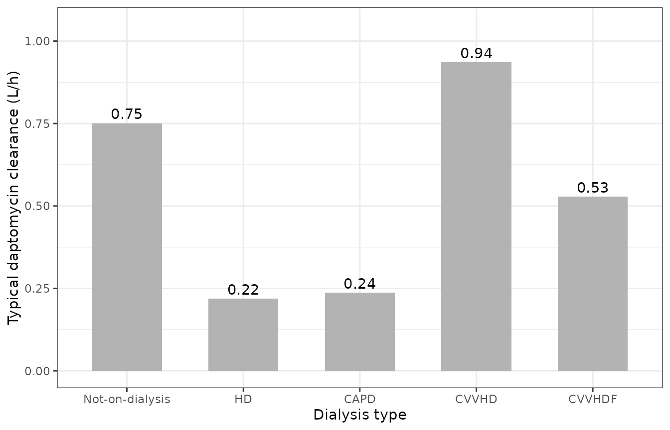
Typical daptomycin clearance by dialysis type. Replicates the central tendency of Figure 4 of Xu 2017 (that figure additionally shows the individual spread).
Validation 2 – structural check against the closed-form solution
A two-compartment model whose model() block defines
cl, vc, q and vp can
be silently rerouted by rxode2 through its analytic solver,
so the explicit ODE system is checked against the closed-form
biexponential solution for a constant-rate infusion of duration
d1 at steady state. This is a pure numerical comparison of
two expressions of the same parameters, so a tight absolute bound is the
right gate.
cvvhdPars <- typicalPk[typicalPk$`Dialysis type` == "CVVHD", ]
CL <- cvvhdPars$CL; VC <- cvvhdPars$Vc; Q <- cvvhdPars$Q2; VP <- cvvhdPars$Vp
D1 <- 0.41
dose <- 500

k10 <- CL / VC; k12 <- Q / VC; k21 <- Q / VP
bsum <- k10 + k12 + k21
alpha <- (bsum + sqrt(bsum^2 - 4 * k10 * k21)) / 2
beta <- (bsum - sqrt(bsum^2 - 4 * k10 * k21)) / 2
rate <- dose / D1
A <- rate / VC * (k21 - alpha) / (alpha * (beta - alpha))
B <- rate / VC * (k21 - beta) / (beta * (alpha - beta))

# Single-dose infusion concentration, on and after the infusion.
ccClosed <- function(tt) {
  ifelse(
    tt <= D1,
    A * (1 - exp(-alpha * tt)) + B * (1 - exp(-beta * tt)),
    A * (1 - exp(-alpha * D1)) * exp(-alpha * (tt - D1)) +
      B * (1 - exp(-beta * D1)) * exp(-beta * (tt - D1))
  )
}

tGrid <- c(0.1, 0.25, 0.41, 0.5, 1, 2, 4, 8, 12, 18, 24)
evCf <- rxode2::et(amt = dose, cmt = "central", rate = -2) |> rxode2::et(tGrid)
# Tight tolerances: the identity is checked to 1e-6 mg/L on a ~60 mg/L peak,
# and the ODE solve at the default rtol leaves ~3e-5 mg/L.
solCf <- rxode2::rxSolve(
  modTypical, withCov(evCf, RRT_CVVHD_STATUS = 1), returnType = "data.frame",
  rtol = 1e-10, atol = 1e-12
)
#> ℹ omega/sigma items treated as zero: 'etalcl', 'etalvc', 'etalq', 'etalvp'
solCf <- solCf[!is.na(solCf$Cc) & solCf$time > 0, ]
solCf$closed <- ccClosed(solCf$time)

stopifnot(
  nrow(solCf) == length(tGrid),
  max(abs(solCf$Cc - solCf$closed)) < 1e-6
)
knitr::kable(
  solCf[, c("time", "Cc", "closed")], digits = 5, row.names = FALSE,
  caption = "ODE solve vs closed-form two-compartment infusion solution (CVVHD typical subject, 500 mg)."
)| time | Cc | closed |
|---|---|---|
| 0.10 | 19.89420 | 19.89420 |
| 0.25 | 45.60209 | 45.60209 |
| 0.41 | 69.19212 | 69.19212 |
| 0.50 | 63.21723 | 63.21723 |
| 1.00 | 46.47317 | 46.47317 |
| 2.00 | 38.39937 | 38.39937 |
| 4.00 | 32.09508 | 32.09508 |
| 8.00 | 22.78759 | 22.78759 |
| 12.00 | 16.17986 | 16.17986 |
| 18.00 | 9.68031 | 9.68031 |
| 24.00 | 5.79167 | 5.79167 |
Validation 3 – dose recovery
For an intravenous drug the area under the curve to infinity times clearance must return the delivered dose. The two sides here use the same drawn parameters, so the difference is pure numerical error and a tight bound is appropriate.
evLong <- rxode2::et(amt = dose, cmt = "central", rate = -2) |>
  rxode2::et(seq(0, 240, by = 0.05))
solLong <- rxode2::rxSolve(
  modTypical, withCov(evLong, RRT_CVVHD_STATUS = 1), returnType = "data.frame"
)
#> ℹ omega/sigma items treated as zero: 'etalcl', 'etalvc', 'etalq', 'etalvp'
solLong <- solLong[!is.na(solLong$Cc), ]
aucObs <- sum(diff(solLong$time) *
  (utils::head(solLong$Cc, -1) + utils::tail(solLong$Cc, -1)) / 2)
aucExtrap <- utils::tail(solLong$Cc, 1) / beta
doseRecovered <- CL * (aucObs + aucExtrap)

c(dose = dose, recovered = doseRecovered, pct_diff = 100 * (doseRecovered / dose - 1))
#>          dose     recovered      pct_diff
#> 500.000000000 499.960494907  -0.007901019
stopifnot(abs(doseRecovered / dose - 1) < 0.005)
Virtual cohort – the 17 CRRT subjects of Xu 2017
Supplementary Table S1 lists every CRRT subject’s body weight, sex and dialysis modality, and main-paper Table 1 gives the subgroup medians for body temperature, the membrane flux distribution and the infection status. That is enough to rebuild the exact cohort the paper simulated, so the virtual population below is the published cohort rather than a resampled one – 9 CVVHD and 8 CVVHDF subjects, well inside the 200-per-arm cap.
Two covariates cannot be resolved at the individual level and are set to their reference (all-zero) state: the per-subject adjudicated diagnosis, and the membrane flux for the CVVHD subgroup (Table 1 records 1 low flux, 2 high flux and 6 not available, without saying which subject is which). All 8 CVVHDF subjects were on a high-flux membrane, so that factor is applied there; it matters, because it raises the realised CVVHDF clearance from 0.528 to 0.72 L/h. See Assumptions and deviations.
subjects <- data.frame(
  id = c(5001, 5002, 5003, 5004, 5005, 5006, 5007, 5008, 5009,
         6001, 6002, 6003, 6004, 6005, 6007, 6008, 6009),
  WT = c(95, 73, 87, 65, 83, 87, 100, 85, 42,
         82, 63, 117, 95, 70, 120, 75, 85),
  SEXF = c(0, 0, 0, 0, 0, 0, 0, 0, 1,
           0, 0, 0, 0, 1, 1, 0, 0),
  modality = c(rep("CVVHD", 9), rep("CVVHDF", 8)),
  stringsAsFactors = FALSE
)
subjects <- subjects |>
  dplyr::mutate(
    RRT_CVVHD_STATUS = as.integer(modality == "CVVHD"),
    RRT_CVVHDF_STATUS = as.integer(modality == "CVVHDF"),
    BODYTEMP = ifelse(modality == "CVVHD", 37.2, 36.8),
    FILT_FLUX_HIGH = as.integer(modality == "CVVHDF"),
    DIS_INFECT_ACTIVE = 1L
  )
knitr::kable(
  subjects, caption = "Xu 2017 supplementary Table S1 (weight, sex, modality) plus the Table 1 subgroup covariates."
)| id | WT | SEXF | modality | RRT_CVVHD_STATUS | RRT_CVVHDF_STATUS | BODYTEMP | FILT_FLUX_HIGH | DIS_INFECT_ACTIVE |
|---|---|---|---|---|---|---|---|---|
| 5001 | 95 | 0 | CVVHD | 1 | 0 | 37.2 | 0 | 1 |
| 5002 | 73 | 0 | CVVHD | 1 | 0 | 37.2 | 0 | 1 |
| 5003 | 87 | 0 | CVVHD | 1 | 0 | 37.2 | 0 | 1 |
| 5004 | 65 | 0 | CVVHD | 1 | 0 | 37.2 | 0 | 1 |
| 5005 | 83 | 0 | CVVHD | 1 | 0 | 37.2 | 0 | 1 |
| 5006 | 87 | 0 | CVVHD | 1 | 0 | 37.2 | 0 | 1 |
| 5007 | 100 | 0 | CVVHD | 1 | 0 | 37.2 | 0 | 1 |
| 5008 | 85 | 0 | CVVHD | 1 | 0 | 37.2 | 0 | 1 |
| 5009 | 42 | 1 | CVVHD | 1 | 0 | 37.2 | 0 | 1 |
| 6001 | 82 | 0 | CVVHDF | 0 | 1 | 36.8 | 1 | 1 |
| 6002 | 63 | 0 | CVVHDF | 0 | 1 | 36.8 | 1 | 1 |
| 6003 | 117 | 0 | CVVHDF | 0 | 1 | 36.8 | 1 | 1 |
| 6004 | 95 | 0 | CVVHDF | 0 | 1 | 36.8 | 1 | 1 |
| 6005 | 70 | 1 | CVVHDF | 0 | 1 | 36.8 | 1 | 1 |
| 6007 | 120 | 1 | CVVHDF | 0 | 1 | 36.8 | 1 | 1 |
| 6008 | 75 | 0 | CVVHDF | 0 | 1 | 36.8 | 1 | 1 |
| 6009 | 85 | 0 | CVVHDF | 0 | 1 | 36.8 | 1 | 1 |
tau24 <- 24
tau48 <- 48
doses <- c(4, 6, 8, 10, 12)

simulateRegimen <- function(dosePerKg, tau) {
  nDose <- ceiling(240 / tau)
  tStart <- (nDose - 1) * tau
  obsGrid <- sort(unique(c(
    seq(tStart, tStart + tau, by = 0.5),
    tStart + c(0.41, 0.75, 1, 1.5, 2, 3), tStart + tau
  )))
  out <- lapply(seq_len(nrow(subjects)), function(i) {
    s <- subjects[i, ]
    ev <- rxode2::et(
      amt = dosePerKg * s$WT, cmt = "central", rate = -2,
      ii = tau, until = tStart
    ) |>
      rxode2::et(obsGrid)
    d <- withCov(
      ev,
      WT = s$WT, SEXF = s$SEXF, BODYTEMP = s$BODYTEMP,
      RRT_CVVHD_STATUS = s$RRT_CVVHD_STATUS,
      RRT_CVVHDF_STATUS = s$RRT_CVVHDF_STATUS,
      FILT_FLUX_HIGH = s$FILT_FLUX_HIGH,
      DIS_INFECT_ACTIVE = s$DIS_INFECT_ACTIVE
    )
    r <- rxode2::rxSolve(modTypical, d, returnType = "data.frame")
    r <- r[!is.na(r$Cc), c("time", "Cc")]
    r$time <- r$time - tStart
    r$id <- s$id
    r$modality <- s$modality
    r$dose_mgkg <- dosePerKg
    r$tau <- tau
    r$amt <- dosePerKg * s$WT
    r[order(r$time), ]
  })
  dplyr::bind_rows(out)
}

conc <- dplyr::bind_rows(c(
  lapply(doses, simulateRegimen, tau = tau24),
  lapply(doses, simulateRegimen, tau = tau48)
)) |>
  dplyr::mutate(
    treatment = sprintf("%s %g mg/kg Q%gh", modality, dose_mgkg, tau)
  )
#> ℹ omega/sigma items treated as zero: 'etalcl', 'etalvc', 'etalq', 'etalvp'
#> ℹ omega/sigma items treated as zero: 'etalcl', 'etalvc', 'etalq', 'etalvp'
#> ℹ omega/sigma items treated as zero: 'etalcl', 'etalvc', 'etalq', 'etalvp'
#> ℹ omega/sigma items treated as zero: 'etalcl', 'etalvc', 'etalq', 'etalvp'
#> ℹ omega/sigma items treated as zero: 'etalcl', 'etalvc', 'etalq', 'etalvp'
#> ℹ omega/sigma items treated as zero: 'etalcl', 'etalvc', 'etalq', 'etalvp'
#> ℹ omega/sigma items treated as zero: 'etalcl', 'etalvc', 'etalq', 'etalvp'
#> ℹ omega/sigma items treated as zero: 'etalcl', 'etalvc', 'etalq', 'etalvp'
#> ℹ omega/sigma items treated as zero: 'etalcl', 'etalvc', 'etalq', 'etalvp'
#> ℹ omega/sigma items treated as zero: 'etalcl', 'etalvc', 'etalq', 'etalvp'
#> ℹ omega/sigma items treated as zero: 'etalcl', 'etalvc', 'etalq', 'etalvp'
#> ℹ omega/sigma items treated as zero: 'etalcl', 'etalvc', 'etalq', 'etalvp'
#> ℹ omega/sigma items treated as zero: 'etalcl', 'etalvc', 'etalq', 'etalvp'
#> ℹ omega/sigma items treated as zero: 'etalcl', 'etalvc', 'etalq', 'etalvp'
#> ℹ omega/sigma items treated as zero: 'etalcl', 'etalvc', 'etalq', 'etalvp'
#> ℹ omega/sigma items treated as zero: 'etalcl', 'etalvc', 'etalq', 'etalvp'
#> ℹ omega/sigma items treated as zero: 'etalcl', 'etalvc', 'etalq', 'etalvp'
#> ℹ omega/sigma items treated as zero: 'etalcl', 'etalvc', 'etalq', 'etalvp'
#> ℹ omega/sigma items treated as zero: 'etalcl', 'etalvc', 'etalq', 'etalvp'
#> ℹ omega/sigma items treated as zero: 'etalcl', 'etalvc', 'etalq', 'etalvp'
#> ℹ omega/sigma items treated as zero: 'etalcl', 'etalvc', 'etalq', 'etalvp'
#> ℹ omega/sigma items treated as zero: 'etalcl', 'etalvc', 'etalq', 'etalvp'
#> ℹ omega/sigma items treated as zero: 'etalcl', 'etalvc', 'etalq', 'etalvp'
#> ℹ omega/sigma items treated as zero: 'etalcl', 'etalvc', 'etalq', 'etalvp'
#> ℹ omega/sigma items treated as zero: 'etalcl', 'etalvc', 'etalq', 'etalvp'
#> ℹ omega/sigma items treated as zero: 'etalcl', 'etalvc', 'etalq', 'etalvp'
#> ℹ omega/sigma items treated as zero: 'etalcl', 'etalvc', 'etalq', 'etalvp'
#> ℹ omega/sigma items treated as zero: 'etalcl', 'etalvc', 'etalq', 'etalvp'
#> ℹ omega/sigma items treated as zero: 'etalcl', 'etalvc', 'etalq', 'etalvp'
#> ℹ omega/sigma items treated as zero: 'etalcl', 'etalvc', 'etalq', 'etalvp'
#> ℹ omega/sigma items treated as zero: 'etalcl', 'etalvc', 'etalq', 'etalvp'
#> ℹ omega/sigma items treated as zero: 'etalcl', 'etalvc', 'etalq', 'etalvp'
#> ℹ omega/sigma items treated as zero: 'etalcl', 'etalvc', 'etalq', 'etalvp'
#> ℹ omega/sigma items treated as zero: 'etalcl', 'etalvc', 'etalq', 'etalvp'
#> ℹ omega/sigma items treated as zero: 'etalcl', 'etalvc', 'etalq', 'etalvp'
#> ℹ omega/sigma items treated as zero: 'etalcl', 'etalvc', 'etalq', 'etalvp'
#> ℹ omega/sigma items treated as zero: 'etalcl', 'etalvc', 'etalq', 'etalvp'
#> ℹ omega/sigma items treated as zero: 'etalcl', 'etalvc', 'etalq', 'etalvp'
#> ℹ omega/sigma items treated as zero: 'etalcl', 'etalvc', 'etalq', 'etalvp'
#> ℹ omega/sigma items treated as zero: 'etalcl', 'etalvc', 'etalq', 'etalvp'
#> ℹ omega/sigma items treated as zero: 'etalcl', 'etalvc', 'etalq', 'etalvp'
#> ℹ omega/sigma items treated as zero: 'etalcl', 'etalvc', 'etalq', 'etalvp'
#> ℹ omega/sigma items treated as zero: 'etalcl', 'etalvc', 'etalq', 'etalvp'
#> ℹ omega/sigma items treated as zero: 'etalcl', 'etalvc', 'etalq', 'etalvp'
#> ℹ omega/sigma items treated as zero: 'etalcl', 'etalvc', 'etalq', 'etalvp'
#> ℹ omega/sigma items treated as zero: 'etalcl', 'etalvc', 'etalq', 'etalvp'
#> ℹ omega/sigma items treated as zero: 'etalcl', 'etalvc', 'etalq', 'etalvp'
#> ℹ omega/sigma items treated as zero: 'etalcl', 'etalvc', 'etalq', 'etalvp'
#> ℹ omega/sigma items treated as zero: 'etalcl', 'etalvc', 'etalq', 'etalvp'
#> ℹ omega/sigma items treated as zero: 'etalcl', 'etalvc', 'etalq', 'etalvp'
#> ℹ omega/sigma items treated as zero: 'etalcl', 'etalvc', 'etalq', 'etalvp'
#> ℹ omega/sigma items treated as zero: 'etalcl', 'etalvc', 'etalq', 'etalvp'
#> ℹ omega/sigma items treated as zero: 'etalcl', 'etalvc', 'etalq', 'etalvp'
#> ℹ omega/sigma items treated as zero: 'etalcl', 'etalvc', 'etalq', 'etalvp'
#> ℹ omega/sigma items treated as zero: 'etalcl', 'etalvc', 'etalq', 'etalvp'
#> ℹ omega/sigma items treated as zero: 'etalcl', 'etalvc', 'etalq', 'etalvp'
#> ℹ omega/sigma items treated as zero: 'etalcl', 'etalvc', 'etalq', 'etalvp'
#> ℹ omega/sigma items treated as zero: 'etalcl', 'etalvc', 'etalq', 'etalvp'
#> ℹ omega/sigma items treated as zero: 'etalcl', 'etalvc', 'etalq', 'etalvp'
#> ℹ omega/sigma items treated as zero: 'etalcl', 'etalvc', 'etalq', 'etalvp'
#> ℹ omega/sigma items treated as zero: 'etalcl', 'etalvc', 'etalq', 'etalvp'
#> ℹ omega/sigma items treated as zero: 'etalcl', 'etalvc', 'etalq', 'etalvp'
#> ℹ omega/sigma items treated as zero: 'etalcl', 'etalvc', 'etalq', 'etalvp'
#> ℹ omega/sigma items treated as zero: 'etalcl', 'etalvc', 'etalq', 'etalvp'
#> ℹ omega/sigma items treated as zero: 'etalcl', 'etalvc', 'etalq', 'etalvp'
#> ℹ omega/sigma items treated as zero: 'etalcl', 'etalvc', 'etalq', 'etalvp'
#> ℹ omega/sigma items treated as zero: 'etalcl', 'etalvc', 'etalq', 'etalvp'
#> ℹ omega/sigma items treated as zero: 'etalcl', 'etalvc', 'etalq', 'etalvp'
#> ℹ omega/sigma items treated as zero: 'etalcl', 'etalvc', 'etalq', 'etalvp'
#> ℹ omega/sigma items treated as zero: 'etalcl', 'etalvc', 'etalq', 'etalvp'
#> ℹ omega/sigma items treated as zero: 'etalcl', 'etalvc', 'etalq', 'etalvp'
#> ℹ omega/sigma items treated as zero: 'etalcl', 'etalvc', 'etalq', 'etalvp'
#> ℹ omega/sigma items treated as zero: 'etalcl', 'etalvc', 'etalq', 'etalvp'
#> ℹ omega/sigma items treated as zero: 'etalcl', 'etalvc', 'etalq', 'etalvp'
#> ℹ omega/sigma items treated as zero: 'etalcl', 'etalvc', 'etalq', 'etalvp'
#> ℹ omega/sigma items treated as zero: 'etalcl', 'etalvc', 'etalq', 'etalvp'
#> ℹ omega/sigma items treated as zero: 'etalcl', 'etalvc', 'etalq', 'etalvp'
#> ℹ omega/sigma items treated as zero: 'etalcl', 'etalvc', 'etalq', 'etalvp'
#> ℹ omega/sigma items treated as zero: 'etalcl', 'etalvc', 'etalq', 'etalvp'
#> ℹ omega/sigma items treated as zero: 'etalcl', 'etalvc', 'etalq', 'etalvp'
#> ℹ omega/sigma items treated as zero: 'etalcl', 'etalvc', 'etalq', 'etalvp'
#> ℹ omega/sigma items treated as zero: 'etalcl', 'etalvc', 'etalq', 'etalvp'
#> ℹ omega/sigma items treated as zero: 'etalcl', 'etalvc', 'etalq', 'etalvp'
#> ℹ omega/sigma items treated as zero: 'etalcl', 'etalvc', 'etalq', 'etalvp'
#> ℹ omega/sigma items treated as zero: 'etalcl', 'etalvc', 'etalq', 'etalvp'
#> ℹ omega/sigma items treated as zero: 'etalcl', 'etalvc', 'etalq', 'etalvp'
#> ℹ omega/sigma items treated as zero: 'etalcl', 'etalvc', 'etalq', 'etalvp'
#> ℹ omega/sigma items treated as zero: 'etalcl', 'etalvc', 'etalq', 'etalvp'
#> ℹ omega/sigma items treated as zero: 'etalcl', 'etalvc', 'etalq', 'etalvp'
#> ℹ omega/sigma items treated as zero: 'etalcl', 'etalvc', 'etalq', 'etalvp'
#> ℹ omega/sigma items treated as zero: 'etalcl', 'etalvc', 'etalq', 'etalvp'
#> ℹ omega/sigma items treated as zero: 'etalcl', 'etalvc', 'etalq', 'etalvp'
#> ℹ omega/sigma items treated as zero: 'etalcl', 'etalvc', 'etalq', 'etalvp'
#> ℹ omega/sigma items treated as zero: 'etalcl', 'etalvc', 'etalq', 'etalvp'
#> ℹ omega/sigma items treated as zero: 'etalcl', 'etalvc', 'etalq', 'etalvp'
#> ℹ omega/sigma items treated as zero: 'etalcl', 'etalvc', 'etalq', 'etalvp'
#> ℹ omega/sigma items treated as zero: 'etalcl', 'etalvc', 'etalq', 'etalvp'
#> ℹ omega/sigma items treated as zero: 'etalcl', 'etalvc', 'etalq', 'etalvp'
#> ℹ omega/sigma items treated as zero: 'etalcl', 'etalvc', 'etalq', 'etalvp'
#> ℹ omega/sigma items treated as zero: 'etalcl', 'etalvc', 'etalq', 'etalvp'
#> ℹ omega/sigma items treated as zero: 'etalcl', 'etalvc', 'etalq', 'etalvp'
#> ℹ omega/sigma items treated as zero: 'etalcl', 'etalvc', 'etalq', 'etalvp'
#> ℹ omega/sigma items treated as zero: 'etalcl', 'etalvc', 'etalq', 'etalvp'
#> ℹ omega/sigma items treated as zero: 'etalcl', 'etalvc', 'etalq', 'etalvp'
#> ℹ omega/sigma items treated as zero: 'etalcl', 'etalvc', 'etalq', 'etalvp'
#> ℹ omega/sigma items treated as zero: 'etalcl', 'etalvc', 'etalq', 'etalvp'
#> ℹ omega/sigma items treated as zero: 'etalcl', 'etalvc', 'etalq', 'etalvp'
#> ℹ omega/sigma items treated as zero: 'etalcl', 'etalvc', 'etalq', 'etalvp'
#> ℹ omega/sigma items treated as zero: 'etalcl', 'etalvc', 'etalq', 'etalvp'
#> ℹ omega/sigma items treated as zero: 'etalcl', 'etalvc', 'etalq', 'etalvp'
#> ℹ omega/sigma items treated as zero: 'etalcl', 'etalvc', 'etalq', 'etalvp'
#> ℹ omega/sigma items treated as zero: 'etalcl', 'etalvc', 'etalq', 'etalvp'
#> ℹ omega/sigma items treated as zero: 'etalcl', 'etalvc', 'etalq', 'etalvp'
#> ℹ omega/sigma items treated as zero: 'etalcl', 'etalvc', 'etalq', 'etalvp'
#> ℹ omega/sigma items treated as zero: 'etalcl', 'etalvc', 'etalq', 'etalvp'
#> ℹ omega/sigma items treated as zero: 'etalcl', 'etalvc', 'etalq', 'etalvp'
#> ℹ omega/sigma items treated as zero: 'etalcl', 'etalvc', 'etalq', 'etalvp'
#> ℹ omega/sigma items treated as zero: 'etalcl', 'etalvc', 'etalq', 'etalvp'
#> ℹ omega/sigma items treated as zero: 'etalcl', 'etalvc', 'etalq', 'etalvp'
#> ℹ omega/sigma items treated as zero: 'etalcl', 'etalvc', 'etalq', 'etalvp'
#> ℹ omega/sigma items treated as zero: 'etalcl', 'etalvc', 'etalq', 'etalvp'
#> ℹ omega/sigma items treated as zero: 'etalcl', 'etalvc', 'etalq', 'etalvp'
#> ℹ omega/sigma items treated as zero: 'etalcl', 'etalvc', 'etalq', 'etalvp'
#> ℹ omega/sigma items treated as zero: 'etalcl', 'etalvc', 'etalq', 'etalvp'
#> ℹ omega/sigma items treated as zero: 'etalcl', 'etalvc', 'etalq', 'etalvp'
#> ℹ omega/sigma items treated as zero: 'etalcl', 'etalvc', 'etalq', 'etalvp'
#> ℹ omega/sigma items treated as zero: 'etalcl', 'etalvc', 'etalq', 'etalvp'
#> ℹ omega/sigma items treated as zero: 'etalcl', 'etalvc', 'etalq', 'etalvp'
#> ℹ omega/sigma items treated as zero: 'etalcl', 'etalvc', 'etalq', 'etalvp'
#> ℹ omega/sigma items treated as zero: 'etalcl', 'etalvc', 'etalq', 'etalvp'
#> ℹ omega/sigma items treated as zero: 'etalcl', 'etalvc', 'etalq', 'etalvp'
#> ℹ omega/sigma items treated as zero: 'etalcl', 'etalvc', 'etalq', 'etalvp'
#> ℹ omega/sigma items treated as zero: 'etalcl', 'etalvc', 'etalq', 'etalvp'
#> ℹ omega/sigma items treated as zero: 'etalcl', 'etalvc', 'etalq', 'etalvp'
#> ℹ omega/sigma items treated as zero: 'etalcl', 'etalvc', 'etalq', 'etalvp'
#> ℹ omega/sigma items treated as zero: 'etalcl', 'etalvc', 'etalq', 'etalvp'
#> ℹ omega/sigma items treated as zero: 'etalcl', 'etalvc', 'etalq', 'etalvp'
#> ℹ omega/sigma items treated as zero: 'etalcl', 'etalvc', 'etalq', 'etalvp'
#> ℹ omega/sigma items treated as zero: 'etalcl', 'etalvc', 'etalq', 'etalvp'
#> ℹ omega/sigma items treated as zero: 'etalcl', 'etalvc', 'etalq', 'etalvp'
#> ℹ omega/sigma items treated as zero: 'etalcl', 'etalvc', 'etalq', 'etalvp'
#> ℹ omega/sigma items treated as zero: 'etalcl', 'etalvc', 'etalq', 'etalvp'
#> ℹ omega/sigma items treated as zero: 'etalcl', 'etalvc', 'etalq', 'etalvp'
#> ℹ omega/sigma items treated as zero: 'etalcl', 'etalvc', 'etalq', 'etalvp'
#> ℹ omega/sigma items treated as zero: 'etalcl', 'etalvc', 'etalq', 'etalvp'
#> ℹ omega/sigma items treated as zero: 'etalcl', 'etalvc', 'etalq', 'etalvp'
#> ℹ omega/sigma items treated as zero: 'etalcl', 'etalvc', 'etalq', 'etalvp'
#> ℹ omega/sigma items treated as zero: 'etalcl', 'etalvc', 'etalq', 'etalvp'
#> ℹ omega/sigma items treated as zero: 'etalcl', 'etalvc', 'etalq', 'etalvp'
#> ℹ omega/sigma items treated as zero: 'etalcl', 'etalvc', 'etalq', 'etalvp'
#> ℹ omega/sigma items treated as zero: 'etalcl', 'etalvc', 'etalq', 'etalvp'
#> ℹ omega/sigma items treated as zero: 'etalcl', 'etalvc', 'etalq', 'etalvp'
#> ℹ omega/sigma items treated as zero: 'etalcl', 'etalvc', 'etalq', 'etalvp'
#> ℹ omega/sigma items treated as zero: 'etalcl', 'etalvc', 'etalq', 'etalvp'
#> ℹ omega/sigma items treated as zero: 'etalcl', 'etalvc', 'etalq', 'etalvp'
#> ℹ omega/sigma items treated as zero: 'etalcl', 'etalvc', 'etalq', 'etalvp'
#> ℹ omega/sigma items treated as zero: 'etalcl', 'etalvc', 'etalq', 'etalvp'
#> ℹ omega/sigma items treated as zero: 'etalcl', 'etalvc', 'etalq', 'etalvp'
#> ℹ omega/sigma items treated as zero: 'etalcl', 'etalvc', 'etalq', 'etalvp'
#> ℹ omega/sigma items treated as zero: 'etalcl', 'etalvc', 'etalq', 'etalvp'
#> ℹ omega/sigma items treated as zero: 'etalcl', 'etalvc', 'etalq', 'etalvp'
#> ℹ omega/sigma items treated as zero: 'etalcl', 'etalvc', 'etalq', 'etalvp'
#> ℹ omega/sigma items treated as zero: 'etalcl', 'etalvc', 'etalq', 'etalvp'
#> ℹ omega/sigma items treated as zero: 'etalcl', 'etalvc', 'etalq', 'etalvp'
#> ℹ omega/sigma items treated as zero: 'etalcl', 'etalvc', 'etalq', 'etalvp'
#> ℹ omega/sigma items treated as zero: 'etalcl', 'etalvc', 'etalq', 'etalvp'
#> ℹ omega/sigma items treated as zero: 'etalcl', 'etalvc', 'etalq', 'etalvp'
#> ℹ omega/sigma items treated as zero: 'etalcl', 'etalvc', 'etalq', 'etalvp'
#> ℹ omega/sigma items treated as zero: 'etalcl', 'etalvc', 'etalq', 'etalvp'
#> ℹ omega/sigma items treated as zero: 'etalcl', 'etalvc', 'etalq', 'etalvp'
nrow(conc)
#> [1] 12750
conc |>
  dplyr::filter(dose_mgkg == 6) |>
  ggplot2::ggplot(ggplot2::aes(time, Cc, group = id, colour = modality)) +
  ggplot2::geom_line(alpha = 0.8) +
  ggplot2::facet_wrap(~ sprintf("Q%gh", tau), scales = "free_x") +
  ggplot2::labs(
    x = "Time since dose (h)", y = "Daptomycin concentration (mg/L)",
    colour = "Modality"
  ) +
  ggplot2::theme_bw()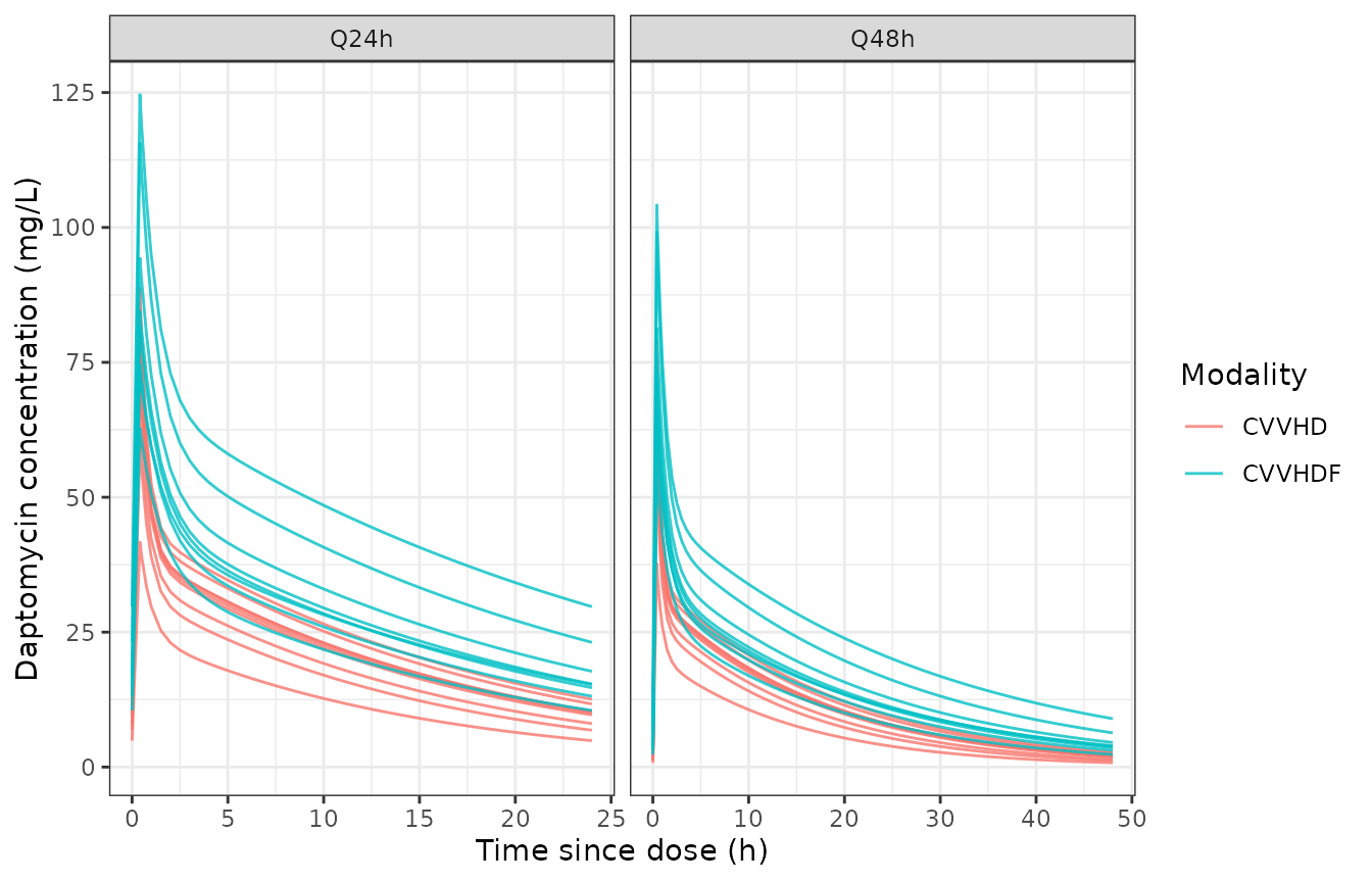
Steady-state daptomycin concentration-time profiles for the 17 CRRT subjects at 6 mg/kg. The left panel covers the Q24h interval and the right panel the Q48h interval, reproducing the shape of Figure 1 of Xu 2017.
PKNCA validation
Non-compartmental analysis is run with PKNCA over the final dosing
interval of each regimen. The concentration frame is filtered only on
!is.na(Cc) so the time-zero record is preserved and the
interval-end record is present for cmin.
concData <- conc |>
  dplyr::filter(!is.na(Cc)) |>
  dplyr::mutate(id = as.character(id))

doseData <- concData |>
  dplyr::group_by(id, treatment) |>
  dplyr::summarise(time = 0, amt = dplyr::first(amt), .groups = "drop") |>
  as.data.frame()

concObj <- PKNCA::PKNCAconc(
  as.data.frame(concData), Cc ~ time | id / treatment
)
doseObj <- PKNCA::PKNCAdose(
  doseData, amt ~ time | id + treatment, route = "intravascular"
)

intervals <- dplyr::bind_rows(
  data.frame(start = 0, end = 24, auclast = TRUE, cmax = TRUE, cmin = TRUE, tmax = TRUE),
  data.frame(start = 24, end = 48, auclast = TRUE, cmax = FALSE, cmin = FALSE, tmax = FALSE)
)

ncaRes <- PKNCA::pk.nca(
  PKNCA::PKNCAdata(concObj, doseObj, intervals = intervals),
  verbose = FALSE
)
ncaTab <- as.data.frame(ncaRes) |>
  dplyr::mutate(
    PPTESTCD = dplyr::case_when(
      PPTESTCD == "auclast" & start == 0 ~ "AUC0-24h",
      PPTESTCD == "auclast" & start == 24 ~ "AUC24-48h",
      TRUE ~ PPTESTCD
    )
  ) |>
  dplyr::filter(!is.na(PPORRES))
head(ncaTab)
#> # A tibble: 6 × 7
#>   id    treatment           start   end PPTESTCD  PPORRES exclude
#>   <chr> <chr>               <dbl> <dbl> <chr>       <dbl> <chr>
#> 1 5001  CVVHD 10 mg/kg Q24h     0    24 AUC0-24h 1001.    <NA>
#> 2 5001  CVVHD 10 mg/kg Q24h     0    24 cmax      141.    <NA>
#> 3 5001  CVVHD 10 mg/kg Q24h     0    24 cmin       19.5   <NA>
#> 4 5001  CVVHD 10 mg/kg Q24h     0    24 tmax        0.410 <NA>
#> 5 5001  CVVHD 10 mg/kg Q48h     0    24 AUC0-24h  796.    <NA>
#> 6 5001  CVVHD 10 mg/kg Q48h     0    24 cmax      126.    <NA>
The Q24h regimens have no 24-48 h window, so the second interval is dropped for those treatments before summarising.
ncaSummary <- ncaTab |>
  dplyr::left_join(
    dplyr::distinct(conc, treatment, modality, dose_mgkg, tau), by = "treatment"
  ) |>
  dplyr::filter(!(tau == 24 & PPTESTCD == "AUC24-48h")) |>
  dplyr::group_by(treatment, modality, dose_mgkg, tau, PPTESTCD) |>
  dplyr::summarise(PPORRES = mean(PPORRES), .groups = "drop")

stopifnot(
  all(c("cmax", "cmin", "AUC0-24h") %in% ncaSummary$PPTESTCD),
  !anyNA(ncaSummary$PPORRES)
)
Comparison against the published Xu 2017 Table 3
Table 3 of Xu 2017 reports the mean AUC, Cmax and Cmin over 100 parametric bootstrap resamples of the individual MAP-Bayes parameter sets. The reproduction here instead uses the published typical parameters conditioned on each subject’s known covariates, so the two sides differ by the individual random effects and by the covariates Table 1 does not resolve per subject; the tolerance is set to 20%, the package’s default.
For the Q24h regimens the paper’s AUCss is the
steady-state AUC over the 24 h interval, compared with the simulated
auc0_24. For Q48h the paper prints AUC0-24h
and AUC24-48h separately.
ref24 <- data.frame(
  modality = rep(c("CVVHD", "CVVHDF"), each = 5),
  dose_mgkg = rep(doses, 2),
  `AUC0-24h` = c(335, 498, 673, 839, 999, 508, 712, 1000, 1203, 1475),
  cmax = c(46, 69, 92, 115, 137, 57, 82, 113, 139, 169),
  cmin = c(6.2, 9.0, 12.0, 15.4, 18.0, 11.0, 15.4, 21.7, 26.5, 32.2),
  check.names = FALSE
) |>
  dplyr::mutate(treatment = sprintf("%s %g mg/kg Q24h", modality, dose_mgkg))

ref48 <- data.frame(
  modality = rep(c("CVVHD", "CVVHDF"), each = 5),
  dose_mgkg = rep(doses, 2),
  `AUC0-24h` = c(272, 404, 542, 684, 799, 383, 558, 759, 936, 1129),
  `AUC24-48h` = c(63, 93, 126, 158, 182, 126, 180, 244, 304, 361),
  cmax = c(42, 62, 82, 104, 124, 49, 73, 98, 121, 147),
  cmin = c(1.2, 1.8, 2.4, 3.1, 3.5, 3.1, 4.5, 6.1, 7.8, 8.8),
  check.names = FALSE
) |>
  dplyr::mutate(treatment = sprintf("%s %g mg/kg Q48h", modality, dose_mgkg))

reference <- dplyr::bind_rows(
  dplyr::select(ref24, treatment, `AUC0-24h`, cmax, cmin),
  dplyr::select(ref48, treatment, `AUC0-24h`, `AUC24-48h`, cmax, cmin)
) |>
  # Long form, dropping the auc24_48 cells that the Q24h regimens do not have.
  tidyr::pivot_longer(
    -treatment, names_to = "PPTESTCD", values_to = "PPORRES", values_drop_na = TRUE
  ) |>
  as.data.frame()
nrow(reference)
#> [1] 70
comparison <- nlmixr2lib::ncaComparisonTable(
  simulated = dplyr::select(ncaSummary, treatment, PPTESTCD, PPORRES),
  reference = reference,
  by = "treatment",
  units = c(
    `AUC0-24h` = "mg*h/L", `AUC24-48h` = "mg*h/L",
    cmax = "mg/L", cmin = "mg/L"
  ),
  tolerance_pct = 20
)
#> Warning: ncaParamLabel(): unknown PKNCA code(s) returned as-is: 'AUC0-24h',
#> 'AUC24-48h'
knitr::kable(
  comparison,
  caption = "Simulated vs published Xu 2017 Table 3 exposures in CVVHD and CVVHDF subjects."
)| NCA parameter | treatment | Reference | Simulated | % diff |
|---|---|---|---|---|
| Cmax (mg/L) | CVVHD 4 mg/kg Q24h | 46 | 48.3 | +4.9% |
| Cmax (mg/L) | CVVHD 6 mg/kg Q24h | 69 | 72.4 | +4.9% |
| Cmax (mg/L) | CVVHD 8 mg/kg Q24h | 92 | 96.5 | +4.9% |
| Cmax (mg/L) | CVVHD 10 mg/kg Q24h | 115 | 121 | +4.9% |
| Cmax (mg/L) | CVVHD 12 mg/kg Q24h | 137 | 145 | +5.7% |
| Cmax (mg/L) | CVVHDF 4 mg/kg Q24h | 57 | 59.2 | +3.9% |
| Cmax (mg/L) | CVVHDF 6 mg/kg Q24h | 82 | 88.9 | +8.4% |
| Cmax (mg/L) | CVVHDF 8 mg/kg Q24h | 113 | 118 | +4.9% |
| Cmax (mg/L) | CVVHDF 10 mg/kg Q24h | 139 | 148 | +6.6% |
| Cmax (mg/L) | CVVHDF 12 mg/kg Q24h | 169 | 178 | +5.2% |
| Cmax (mg/L) | CVVHD 4 mg/kg Q48h | 42 | 43.4 | +3.3% |
| Cmax (mg/L) | CVVHD 6 mg/kg Q48h | 62 | 65.1 | +4.9% |
| Cmax (mg/L) | CVVHD 8 mg/kg Q48h | 82 | 86.7 | +5.8% |
| Cmax (mg/L) | CVVHD 10 mg/kg Q48h | 104 | 108 | +4.3% |
| Cmax (mg/L) | CVVHD 12 mg/kg Q48h | 124 | 130 | +4.9% |
| Cmax (mg/L) | CVVHDF 4 mg/kg Q48h | 49 | 50.8 | +3.7% |
| Cmax (mg/L) | CVVHDF 6 mg/kg Q48h | 73 | 76.2 | +4.4% |
| Cmax (mg/L) | CVVHDF 8 mg/kg Q48h | 98 | 102 | +3.7% |
| Cmax (mg/L) | CVVHDF 10 mg/kg Q48h | 121 | 127 | +5.0% |
| Cmax (mg/L) | CVVHDF 12 mg/kg Q48h | 147 | 152 | +3.7% |
| Cmin (mg/L) | CVVHD 4 mg/kg Q24h | 6.2 | 6.25 | +0.8% |
| Cmin (mg/L) | CVVHD 6 mg/kg Q24h | 9 | 9.38 | +4.2% |
| Cmin (mg/L) | CVVHD 8 mg/kg Q24h | 12 | 12.5 | +4.2% |
| Cmin (mg/L) | CVVHD 10 mg/kg Q24h | 15.4 | 15.6 | +1.5% |
| Cmin (mg/L) | CVVHD 12 mg/kg Q24h | 18 | 18.8 | +4.2% |
| Cmin (mg/L) | CVVHDF 4 mg/kg Q24h | 11 | 11.6 | +5.7% |
| Cmin (mg/L) | CVVHDF 6 mg/kg Q24h | 15.4 | 17.4 | +13.3% |
| Cmin (mg/L) | CVVHDF 8 mg/kg Q24h | 21.7 | 23.3 | +7.2% |
| Cmin (mg/L) | CVVHDF 10 mg/kg Q24h | 26.5 | 29.1 | +9.7% |
| Cmin (mg/L) | CVVHDF 12 mg/kg Q24h | 32.2 | 34.9 | +8.3% |
| Cmin (mg/L) | CVVHD 4 mg/kg Q48h | 1.2 | 1.24 | +3.4% |
| Cmin (mg/L) | CVVHD 6 mg/kg Q48h | 1.8 | 1.86 | +3.4% |
| Cmin (mg/L) | CVVHD 8 mg/kg Q48h | 2.4 | 2.48 | +3.4% |
| Cmin (mg/L) | CVVHD 10 mg/kg Q48h | 3.1 | 3.1 | +0.1% |
| Cmin (mg/L) | CVVHD 12 mg/kg Q48h | 3.5 | 3.72 | +6.4% |
| Cmin (mg/L) | CVVHDF 4 mg/kg Q48h | 3.1 | 3.05 | -1.5% |
| Cmin (mg/L) | CVVHDF 6 mg/kg Q48h | 4.5 | 4.58 | +1.7% |
| Cmin (mg/L) | CVVHDF 8 mg/kg Q48h | 6.1 | 6.1 | +0.1% |
| Cmin (mg/L) | CVVHDF 10 mg/kg Q48h | 7.8 | 7.63 | -2.2% |
| Cmin (mg/L) | CVVHDF 12 mg/kg Q48h | 8.8 | 9.16 | +4.1% |
| AUC0-24h (mg*h/L) | CVVHD 4 mg/kg Q24h | 335 | 339 | +1.2% |
| AUC0-24h (mg*h/L) | CVVHD 6 mg/kg Q24h | 498 | 508 | +2.1% |
| AUC0-24h (mg*h/L) | CVVHD 8 mg/kg Q24h | 673 | 678 | +0.7% |
| AUC0-24h (mg*h/L) | CVVHD 10 mg/kg Q24h | 839 | 847 | +1.0% |
| AUC0-24h (mg*h/L) | CVVHD 12 mg/kg Q24h | 999 | 1020 | +1.8% |
| AUC0-24h (mg*h/L) | CVVHDF 4 mg/kg Q24h | 508 | 519 | +2.1% |
| AUC0-24h (mg*h/L) | CVVHDF 6 mg/kg Q24h | 712 | 778 | +9.3% |
| AUC0-24h (mg*h/L) | CVVHDF 8 mg/kg Q24h | 1000 | 1040 | +3.8% |
| AUC0-24h (mg*h/L) | CVVHDF 10 mg/kg Q24h | 1200 | 1300 | +7.8% |
| AUC0-24h (mg*h/L) | CVVHDF 12 mg/kg Q24h | 1480 | 1560 | +5.5% |
| AUC0-24h (mg*h/L) | CVVHD 4 mg/kg Q48h | 272 | 274 | +0.8% |
| AUC0-24h (mg*h/L) | CVVHD 6 mg/kg Q48h | 404 | 411 | +1.8% |
| AUC0-24h (mg*h/L) | CVVHD 8 mg/kg Q48h | 542 | 548 | +1.1% |
| AUC0-24h (mg*h/L) | CVVHD 10 mg/kg Q48h | 684 | 685 | +0.2% |
| AUC0-24h (mg*h/L) | CVVHD 12 mg/kg Q48h | 799 | 822 | +2.9% |
| AUC0-24h (mg*h/L) | CVVHDF 4 mg/kg Q48h | 383 | 391 | +2.0% |
| AUC0-24h (mg*h/L) | CVVHDF 6 mg/kg Q48h | 558 | 586 | +5.0% |
| AUC0-24h (mg*h/L) | CVVHDF 8 mg/kg Q48h | 759 | 781 | +2.9% |
| AUC0-24h (mg*h/L) | CVVHDF 10 mg/kg Q48h | 936 | 976 | +4.3% |
| AUC0-24h (mg*h/L) | CVVHDF 12 mg/kg Q48h | 1130 | 1170 | +3.8% |
| AUC24-48h (mg*h/L) | CVVHD 4 mg/kg Q48h | 63 | 64.8 | +2.8% |
| AUC24-48h (mg*h/L) | CVVHD 6 mg/kg Q48h | 93 | 97.2 | +4.5% |
| AUC24-48h (mg*h/L) | CVVHD 8 mg/kg Q48h | 126 | 130 | +2.8% |
| AUC24-48h (mg*h/L) | CVVHD 10 mg/kg Q48h | 158 | 162 | +2.5% |
| AUC24-48h (mg*h/L) | CVVHD 12 mg/kg Q48h | 182 | 194 | +6.8% |
| AUC24-48h (mg*h/L) | CVVHDF 4 mg/kg Q48h | 126 | 128 | +1.7% |
| AUC24-48h (mg*h/L) | CVVHDF 6 mg/kg Q48h | 180 | 192 | +6.8% |
| AUC24-48h (mg*h/L) | CVVHDF 8 mg/kg Q48h | 244 | 256 | +5.1% |
| AUC24-48h (mg*h/L) | CVVHDF 10 mg/kg Q48h | 304 | 320 | +5.4% |
| AUC24-48h (mg*h/L) | CVVHDF 12 mg/kg Q48h | 361 | 385 | +6.5% |
attr(comparison, "footnote")
#> NULL
# ncaComparisonTable() returns the percent-difference column as formatted
# character ("+4.9%"), so strip the sign and unit before comparing.
pctDiff <- as.numeric(sub("%$", "", sub("^\\+", "", comparison[["% diff"]])))
stopifnot(
  # Every published cell of Table 3 is represented.
  nrow(comparison) == 70L,
  !anyNA(pctDiff),
  # Structural: a mis-transcribed clearance, volume, dose or infusion duration
  # moves the whole distribution by tens of percent and blows this instantly.
  abs(median(pctDiff)) < 5,
  # Envelope: bounds the subjects whose unresolved covariates matter most.
  # The cohort is the published one and the random effects are zeroed, so
  # these numbers are deterministic and the bounds can be tight.
  stats::quantile(abs(pctDiff), 0.9) < 8,
  max(abs(pctDiff)) < 15,
  # The model must not systematically UNDER-predict: every simulated cell
  # should sit at or above the paper's mean, because the covariates that
  # could not be resolved per subject all act to raise clearance.
  min(pctDiff) > -5
)
Dosing-interval conclusion of Xu 2017
The paper’s clinical conclusion is that Q24h dosing keeps steady-state exposure inside the efficacy-to-safety window in CRRT patients, whereas Q48h dosing drops below the lower efficacy boundary on the second day at every dose from 4 to 12 mg/kg. The efficacy reference is an AUC0-24h of 465-761 mgh/L and the safety threshold an AUC0-24h of 1422 mgh/L (Methods, “Simulations and references for drug exposure”). The simulated exposures reproduce that conclusion.
auc <- ncaSummary |>
  dplyr::filter(PPTESTCD %in% c("AUC0-24h", "AUC24-48h")) |>
  dplyr::select(modality, dose_mgkg, tau, PPTESTCD, PPORRES) |>
  tidyr::pivot_wider(names_from = PPTESTCD, values_from = PPORRES) |>
  dplyr::rename(auc0_24 = `AUC0-24h`, auc24_48 = `AUC24-48h`)

day2 <- auc |> dplyr::filter(tau == 48)
stopifnot(
  # Q48h day 2 falls below the lower efficacy boundary at EVERY dose level.
  nrow(day2) == 10L,
  all(day2$auc24_48 < 465)
)

q24 <- auc |> dplyr::filter(tau == 24)
stopifnot(
  # Q24h keeps CVVHD inside the efficacy-to-safety window from 6 mg/kg up.
  all(q24$auc0_24[q24$modality == "CVVHD" & q24$dose_mgkg >= 6] > 465),
  all(q24$auc0_24[q24$modality == "CVVHD"] < 1422)
)

ggplot2::ggplot(auc, ggplot2::aes(dose_mgkg, auc0_24, colour = modality)) +
  ggplot2::geom_line() +
  ggplot2::geom_point() +
  ggplot2::geom_line(
    data = day2, ggplot2::aes(y = auc24_48, colour = modality), linetype = "dashed"
  ) +
  ggplot2::geom_hline(yintercept = c(465, 761), linetype = "dotted") +
  ggplot2::geom_hline(yintercept = 1422, linetype = "longdash") +
  ggplot2::facet_wrap(~ sprintf("Q%gh", tau)) +
  ggplot2::labs(
    x = "Dose (mg/kg)", y = "AUC over the 24 h window (mg*h/L)",
    colour = "Modality",
    caption = paste(
      "Solid: AUC0-24h. Dashed (Q48h panel): AUC24-48h.",
      "Dotted: 465-761 efficacy range. Long-dash: 1422 safety threshold."
    )
  ) +
  ggplot2::theme_bw()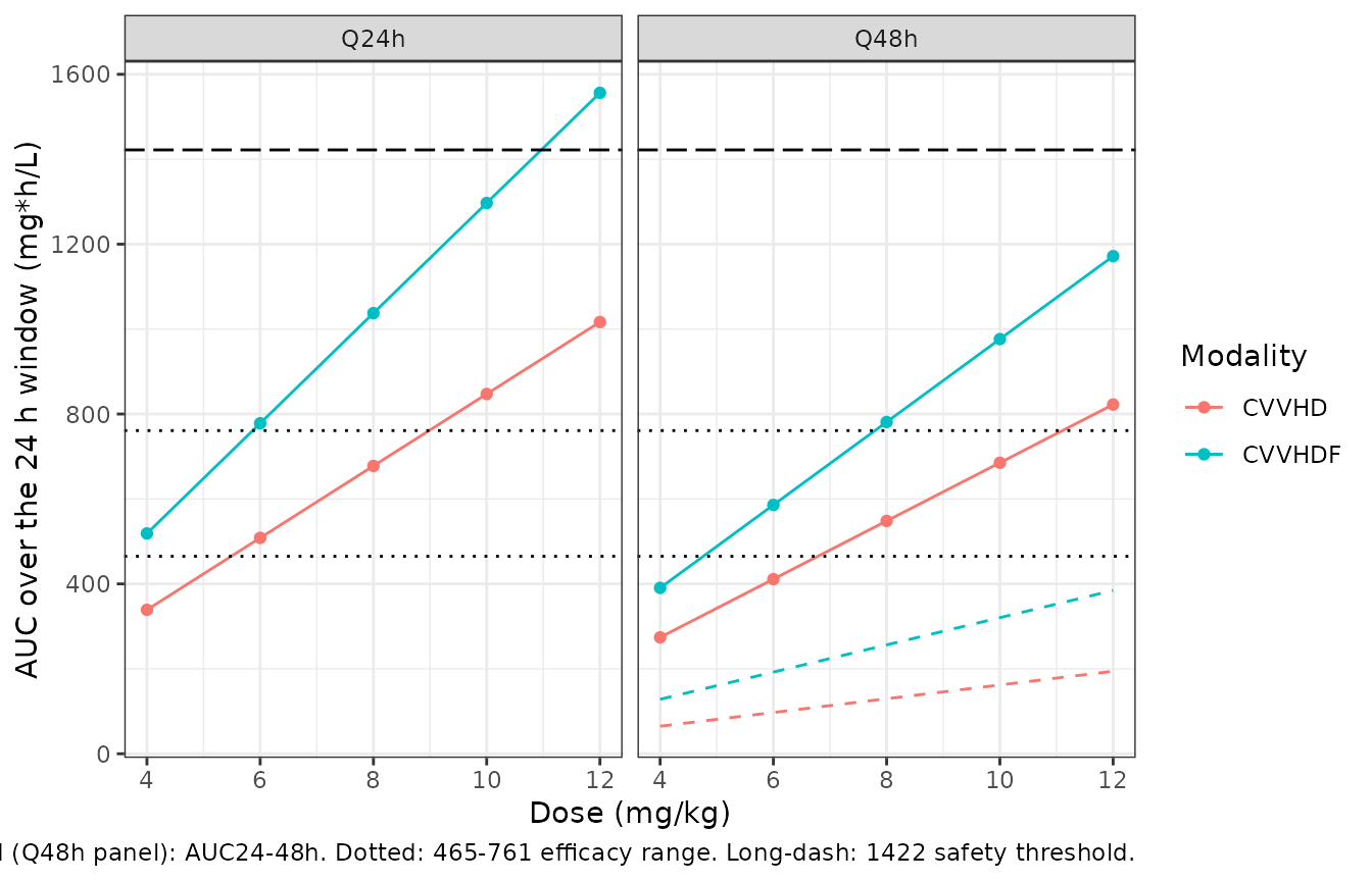
Assumptions and deviations
-
Unknown-dialysis-status stratum omitted. Xu 2017 Eq
1 lists a fifth clearance level,
theta 1= 0.599 L/h, for “patients on unknown dialysis”. The Results state that the three subjects with unknown dialysis status were excluded from this analysis, so no subject in the fitted dataset occupies that stratum, and its 74% relative standard error reflects that. It is therefore not encoded as a covariate column; adding a column no analysed subject carries would fail the registry’s structural-cleanliness check. Users needing that level should treat the value as inherited from the Chaves 2014 base model. -
Inter-individual variance scale. Supplementary
Table S2’s variance cells are ambiguous as printed; the variance reading
is adopted after the three checks set out under “Reading the
supplementary Table S2 variance cells” above. The
CV=andSD=annotations in those cells are arithmetic artefacts of the estimate’s standard error and are not used. -
CL-Vc covariance derived, not printed. Table S2
prints the correlation (r = 0.52) for the CL-V1 covariance but the
estimate cell is blank, so the covariance is recovered as
0.52 * sqrt(0.296 * 0.654)= 0.2288. The correlation and the two variances over-determine the covariance, so this is a solve rather than an assumption. -
Residual SDs derived from printed variances. Table
S2 reports
sigma^2 addrather than SDs; the model takes sqrt(2.07) and sqrt(5.31). - Per-subject diagnosis and CVVHD membrane flux not resolvable. Table 1 gives the IEAC-diagnosis and membrane-flux distributions per subgroup but not per subject, so the cohort simulation sets all five diagnosis indicators to 0 (the unadjudicated reference level, which covers 73% of the pooled dataset) and leaves the CVVHD membrane at “not available”. The CVVHDF subgroup is set to high flux because Table 1 records 8 of 8. This is the main reason the reproduction of Table 3 is not exact.
- Body temperature taken as the subgroup median. Table S1 does not list per-subject temperature, so the CVVHD and CVVHDF medians from Table 1 (37.2 and 36.8 degC) are used. Across the observed 35.1-40.1 degC range the term moves clearance by under 20%, and within the CRRT subgroups by under 5%.
- Paper’s simulation method differs. Xu 2017 simulated from 100 parametric bootstrap resamples of the individual MAP-Bayes parameter sets, which the model file cannot reproduce because those individual estimates are a property of the fit rather than of the model. The comparison here uses the published typical parameters conditioned on each subject’s known covariates.
-
Creatinine-clearance assay not named. The source
writes only “creatinine clearance at baseline (CLC0)” in mL/min with a
reference of 80 mL/min and does not identify the estimating equation.
The
CRCLcolumn is therefore raw, un-normalised mL/min. - No errata found. A search of the journal’s article landing page and PubMed returned no correction, erratum or author notice for doi:10.1111/bcp.13131.
- Non-linear PD, bacterial-kill and target-attainment layers are out of scope. Xu 2017 compares simulated exposures to fixed efficacy and safety reference values taken from earlier publications; it fits no PD model, so none is encoded.