Belzutifan (Marathe 2023)

Model and source

• Citation: Marathe DD, Jauslin PM, Kleijn HJ, de Miranda Silva C, Chain A, Bateman T, Shaw PM, Abraham AK, Kauh EA, Liu Y, Perini RF, de Alwis DP, Jain L. Population pharmacokinetic analyses for belzutifan to inform dosing considerations and labeling. CPT Pharmacometrics Syst Pharmacol. 2023;12(10):1499-1510. doi:10.1002/psp4.13028
• Description: Two-compartment population PK model for oral belzutifan (Welireg, a hypoxia-inducible factor 2 alpha inhibitor) in 239 pooled subjects across four phase I studies and one pivotal phase II study: 83 healthy participants, 74 patients with advanced renal cell carcinoma, 21 with other advanced solid tumors, and 61 with von Hippel-Lindau disease-associated RCC. First-order absorption with an absorption lag and linear elimination from the central compartment. Body weight scales clearances (shared exponent on CL/F and Q/F) and volumes (shared exponent on V2/F and V3/F); age scales CL/F and V2/F; fed state and the final market formulation each slow the absorption rate constant; and the polymorphic UGT2B17 and CYP2C19 metabolizer phenotypes shift CL/F, with UGT2B17 poor metabolizers additionally showing 11% higher relative bioavailability. Residual variability is split into healthy-participant and patient strata.
• Article: https://doi.org/10.1002/psp4.13028
• Supplement (figures S1-S3, tables S1-S5): https://doi.org/10.1002/psp4.13028, Supporting Information
• Supplement 2 contains the verbatim final-model NONMEM control stream, which fixes every covariate branch, reference level, missing-data sentinel, and the S2 = V2/1000 concentration scaling used below.

Belzutifan (Welireg) is an oral inhibitor of hypoxia-inducible factor 2 alpha, approved for von Hippel-Lindau (VHL) disease-associated renal cell carcinoma (RCC), central nervous system hemangioblastomas, and pancreatic neuroendocrine tumors. It is metabolized primarily by the polymorphic enzymes UGT2B17 and CYP2C19, and the headline finding of this analysis is that dual UGT2B17 / CYP2C19 poor metabolizers (PMs) are predicted to have a 3.2-fold higher steady-state AUC than UGT2B17 extensive metabolizers who are CYP2C19 non-PMs.

Population

The model was fit to 5291 measurable plasma concentrations from 239 participants pooled across four phase I studies and one pivotal phase II study (Marathe 2023 Table 1, Table S2). The cohort was 43.9% male, with median (range) age 55 years (19-84) and median body weight 73.6 kg (42.1-165.8). By disease state it comprised 83 healthy participants (34.7%), 74 patients with advanced RCC (31.0%), 21 with other advanced solid tumors (8.8%), and 61 with VHL-RCC (25.5%). Race was 71.5% White, 15.9% Asian, 9.6% Black, and 84.5% were not Hispanic or Latino. Median eGFR was 77.5 mL/min/1.73m^2 (19.6-171.2); by category 80 participants had normal renal function, 104 mild and 52 moderate impairment, and 1 severe. Hepatic function by NCI-ODWG index was normal in 226, mild in 12, and moderate in 1.

Pharmacogenetic phenotypes (Table S2) were, for UGT2B17: 46 poor (19.2%), 98 intermediate (41.0%), 84 extensive (35.1%), 11 missing; and for CYP2C19: 19 poor (7.9%), 65 intermediate, 96 extensive, 42 rapid, 6 ultrarapid, 11 missing. Ten subjects were UGT2B17 / CYP2C19 dual PMs, all from Study 7 – there were no dual PMs in either patient study (Studies 1 and 4).

Doses spanned 20-240 mg once daily plus a 120 mg twice-daily arm in the Study 1 dose escalation, with single doses of 40, 120, and 200 mg in the clinical pharmacology studies. The recommended clinical dosage is 120 mg orally once daily.

The same information is available programmatically via the model’s population metadata (readModelDb("Marathe_2023_belzutifan")()$population – readModelDb() returns the model function, so the trailing () evaluates it to the model object whose $population element holds this list).

Source trace

The per-parameter origin is recorded as an in-file comment next to each ini() entry in inst/modeldb/specificDrugs/Marathe_2023_belzutifan.R. The table below collects them in one place for review.

Equation / parameter	Value	Source location
lka	log(2.40) 1/h	Table 2, “KA (/h)”
lcl	log(5.63) L/h	Table 2, “CL/F (L/h)”
lvc	log(85.4) L	Table 2, “V2/F (L)”
lq	log(5.37) L/h	Table 2, “Q/F (L/h)”
lvp	log(30.38) L	Table 2, “V3/F (L)”
ltlag	log(0.16) h	Table 2, “ALAG (h)”
lfdepot	fixed(log(1))	Table 2 caption, F = 1 * (1 + F-UGT2B17P); supplement 2 F1 = 1 * F1UGT2B17P
e_wt_cl_q	0.65	Table 2, “CL-WT”; shared by CL/F and Q/F per Results
e_wt_vc_vp	1.06	Table 2, “V-WT”; shared by V2/F and V3/F per Results
e_age_cl	-0.36	Table 2, “CL-AGE”
e_age_vc	-0.20	Table 2, “V-AGE”
e_fed_ka	-0.88	Table 2, “KA-FED”; Table 3 gives -87.6%
e_form_belz_fmf_ka	-0.47	Table 2, “KA-FORM”; Table 3 gives -47.4%
e_ugt2b17_em_cl	0.39	Table 2, “CL-UGT2B17 extensive metabolizers”; Table 3 +39.1%
e_ugt2b17_pm_cl	-0.24	Table 2, “CL-UGT2B17 poor metabolizers”; Table 3 -24.2%
e_cyp2c19_pm_cl	-0.36	Table 2, “CL-CYP2C19 poor metabolizers”; Table 3 -36.0%
e_ugt2b17_pm_fdepot	0.11	Table 2, “F-UGT2B17 poor metabolizers”; Table 3 F 1 -> 1.11
etalcl, etalvc, etalvp variances	0.15, 0.013, 0.19	Table 2, “Random effects” (IIV on CL/F, V2/F, V3/F)
etalcl/etalvc/etalvp covariances	derived	Table 2 note: eta correlations 0.40 (CL-V2), 0.54 (CL-V3), 0.38 (V2-V3); covariance = rho * sqrt(var1 * var2)
etalka	1.15	Table 2, “IIV on KA”
propSd_hv	0.26	Table 2, “RESHV”; EPS = 1 FIX
propSd_pt	0.29	Table 2, “RES PAT”; EPS = 1 FIX
Reference body weight 73.64 kg	n/a	Supplement 2 control stream, CLWT = ((WT/73.64)**THETA(10))
Reference age 55 years	n/a	Supplement 2 control stream, CLAGE = ((AGE/55)**THETA(18))
2-compartment structure, first-order absorption + lag	n/a	Results “Base model”; supplement 2 $SUBROUTINE ADVAN4 TRANS4
Cc <- 1000 * central / vc (ng/mL)	n/a	Supplement 2 control stream, S2 = V2/1000
Residual error switched by study	n/a	Supplement 2, PROP = THETA(8) IF (STUDY.EQ.1.OR.STUDY.EQ.4)

Two model choices deserve emphasis because they are easy to get wrong:

1. $SIGMA is fixed to 1 and the proportional error magnitude is carried by a THETA (W = IPRED * PROP, Y = IPRED + W * ERR(1)). The reported RESHV = 0.26 and RES PAT = 0.29 are therefore already proportional standard deviations – no square root is taken.
2. Q/F carries no IIV. The control stream reads Q = THETA(3) * CLWT with no ETA, so only CL/F, V2/F, V3/F, and KA have between-subject variability.

mod <- readModelDb("Marathe_2023_belzutifan")

Covariate-equation verification (Table S4)

Before any ODE solving, the covariate equations can be checked directly against Marathe 2023 Table S4, which tabulates CL/F and V2/F at the 5th, 25th, 50th, 75th, and 95th percentiles of body weight and of age. Solving the packaged model with omega = NA (typical values, no between-subject variability) and reading back the model’s own cl and vc gives an end-to-end check of the power-covariate forms and their reference values.

# Reference phenotype: UGT2B17 intermediate, CYP2C19 non-poor, fasted, FFP,
# patient (matching the Table S4 reference subject).
ref_covs <- function(df) {
  df |>
    mutate(
      FED = 0, FORM_BELZ_FMF = 0,
      UGT2B17_EM = 0, UGT2B17_PM = 0, CYP2C19_PM = 0,
      DIS_HEALTHY = 0
    )
}

s4_grid <- bind_rows(
  tibble(
    sweep = "Body weight (kg)",
    level = c("p5", "p25", "median", "p75", "p95"),
    WT    = c(47.9, 61.5, 73.6, 90.1, 118.4),
    AGE   = 55
  ),
  tibble(
    sweep = "Age (years)",
    level = c("p5", "p25", "median", "p75", "p95"),
    WT    = 73.64,
    AGE   = c(26, 43, 55, 63, 74)
  )
) |>
  ref_covs() |>
  mutate(id = row_number())

# One dose and one observation per covariate combination is enough to read the
# model-computed cl and vc back out.
s4_events <- bind_rows(
  s4_grid |> mutate(time = 0, amt = 120, evid = 1L, cmt = "depot"),
  s4_grid |> mutate(time = 1, amt = NA_real_, evid = 0L, cmt = "central")
) |>
  arrange(id, time, evid)

s4_sim <- rxode2::rxSolve(
  mod, s4_events, omega = NA, keep = c("sweep", "level")
) |>
  as.data.frame()
#> ℹ parameter labels from comments will be replaced by 'label()'
#> Warning: multi-subject simulation without without 'omega'

s4_published <- tibble(
  sweep = rep(c("Body weight (kg)", "Age (years)"), each = 5),
  level = rep(c("p5", "p25", "median", "p75", "p95"), 2),
  cl_pub = c(4.26, 5.01, 5.63, 6.41, 7.65,
             7.37, 6.15, 5.63, 5.37, 5.05),
  vc_pub = c(54.2, 70.5, 85.4, 105.7, 141.1,
             99.6, 89.8, 85.4, 83.1, 80.3)
)

s4_cmp <- s4_sim |>
  group_by(sweep, level) |>
  summarise(cl_sim = mean(cl), vc_sim = mean(vc), .groups = "drop") |>
  right_join(s4_published, by = c("sweep", "level")) |>
  mutate(
    cl_pct = 100 * (cl_sim - cl_pub) / cl_pub,
    vc_pct = 100 * (vc_sim - vc_pub) / vc_pub
  )

# Strict gate: every Table S4 cell must reproduce within 1%.
stopifnot(max(abs(s4_cmp$cl_pct)) < 1, max(abs(s4_cmp$vc_pct)) < 1)

s4_cmp |>
  mutate(across(c(cl_sim, vc_sim), \(x) round(x, 2)),
         across(c(cl_pct, vc_pct), \(x) round(x, 2))) |>
  rename(
    "Covariate sweep"    = sweep,
    "Percentile"         = level,
    "CL/F simulated"     = cl_sim,
    "CL/F Table S4"      = cl_pub,
    "CL/F % diff"        = cl_pct,
    "V2/F simulated"     = vc_sim,
    "V2/F Table S4"      = vc_pub,
    "V2/F % diff"        = vc_pct
  ) |>
  knitr::kable(
    caption = paste(
      "Reproduces Marathe 2023 Table S4: CL/F and V2/F across body-weight and",
      "age percentiles. All cells agree within 1%."
    )
  )

Reproduces Marathe 2023 Table S4: CL/F and V2/F across body-weight and age percentiles. All cells agree within 1%.

Covariate sweep	Percentile	CL/F simulated	V2/F simulated	CL/F Table S4	V2/F Table S4	CL/F % diff	V2/F % diff
Age (years)	median	5.63	85.40	5.63	85.4	0.00	0.00
Age (years)	p25	6.15	89.71	6.15	89.8	0.03	-0.10
Age (years)	p5	7.37	99.21	7.37	99.6	0.04	-0.40
Age (years)	p75	5.36	83.11	5.37	83.1	-0.16	0.01
Age (years)	p95	5.06	80.48	5.05	80.3	0.19	0.22
Body weight (kg)	median	5.63	85.35	5.63	85.4	-0.04	-0.06
Body weight (kg)	p25	5.01	70.55	5.01	70.5	-0.04	0.08
Body weight (kg)	p5	4.26	54.13	4.26	54.2	-0.07	-0.12
Body weight (kg)	p75	6.42	105.76	6.41	105.7	0.14	0.06
Body weight (kg)	p95	7.67	141.28	7.65	141.1	0.21	0.13

Virtual cohorts

Original observed data are not publicly available. The simulations below use two virtual populations.

Cohort 1 – typical-patient phenotype scenarios. Marathe 2023 Table 4 was produced by univariate simulation of a single typical VHL-RCC patient, with covariates held fixed and only the UGT2B17 / CYP2C19 phenotype changed. The Table 4 note defines that reference patient exactly: age 41 years, body weight 74 kg, UGT2B17 intermediate metabolizer, CYP2C19 non-PM, 120 mg once daily in the fasted state using the FFP formulation. Reproducing it needs no distributional assumptions at all, which makes it the primary validation target here.

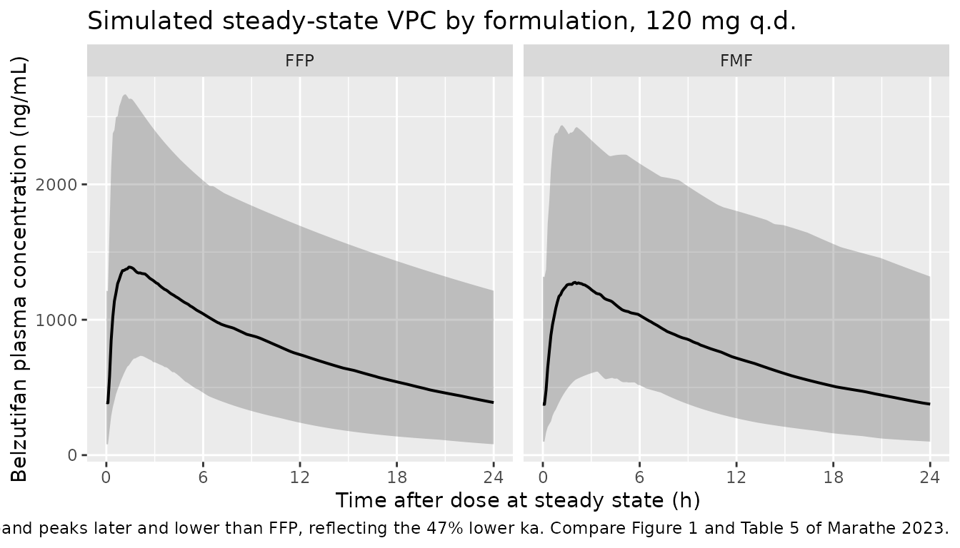
Cohort 2 – the Study 4 VHL-RCC cohort. Table 5 reports steady-state derived parameters for the 61 patients of Study 4, each used 10 times to make 610 virtual patients, once with the covariate formulation set to FFP and once to FMF. Study-4-specific demographics are not published (Table S2 is pooled across all five studies), so this cohort is reconstructed from the Table 4 typical values as distribution centres plus the pooled Table S2 ranges and phenotype frequencies. It is capped at 200 subjects per formulation arm.

set.seed(20231001)

n_days   <- 21L                     # dose to steady state
last_dose <- (n_days - 1L) * 24     # time of the final dose (h)
tau      <- 24                      # dosing interval (h)

# Build a steady-state q.d. event table from a per-subject covariate frame.
# `id_offset` keeps IDs disjoint when several cohorts are bind_rows()-ed:
# rxSolve treats id as the subject key, and duplicate ids across cohorts are
# silently merged into one subject receiving the summed dose.
belz_events <- function(covs, dose = 120, obs_by = 0.1, id_offset = 0L) {
  covs <- covs |> mutate(id = id_offset + row_number())
  doses <- covs |>
    tidyr::expand_grid(time = seq(0, last_dose, by = tau)) |>
    mutate(amt = dose, evid = 1L, cmt = "depot")
  obs <- covs |>
    tidyr::expand_grid(time = last_dose + seq(0, tau, by = obs_by)) |>
    mutate(amt = NA_real_, evid = 0L, cmt = "central")
  # evid = 0 sorts before evid = 1 at identical times, so the observation at
  # the final dose time is the pre-dose trough (Cmin,ss).
  bind_rows(doses, obs) |> arrange(id, time, evid)
}

# --- Cohort 1: the five Table 4 phenotype scenarios --------------------------
pheno <- tibble::tribble(
  ~treatment,                 ~UGT2B17_EM, ~UGT2B17_PM, ~CYP2C19_PM,
  "UGT2B17 IM (reference)",             0,           0,           0,
  "UGT2B17 EM",                         1,           0,           0,
  "UGT2B17 PM",                         0,           1,           0,
  "CYP2C19 PM",                         0,           0,           1,
  "UGT2B17 PM + CYP2C19 PM",            0,           1,           1
) |>
  mutate(WT = 74, AGE = 41, FED = 0, FORM_BELZ_FMF = 0, DIS_HEALTHY = 0)

events_typ <- belz_events(pheno, obs_by = 0.05)

# --- Cohort 2: reconstructed Study 4 VHL-RCC cohort, FFP and FMF arms -------
n_arm <- 200L

# Pooled Table S2 phenotype frequencies among non-missing subjects
# (UGT2B17: 46 PM / 98 IM / 84 EM of 228; CYP2C19: 19 PM of 228). The missing
# sentinel maps onto the reference level exactly as the control stream does.
ugt_draw <- sample(
  c("PM", "IM", "EM"), n_arm, replace = TRUE,
  prob = c(46, 98, 84) / 228
)
# Table S2 footnote b: there were NO UGT2B17/CYP2C19 dual PMs in the patient
# studies (Studies 1 and 4), so CYP2C19 PM status is drawn only among
# non-UGT2B17-PM subjects.
cyp_draw <- ifelse(
  ugt_draw == "PM", 0L,
  rbinom(n_arm, 1, 19 / 228)
)

vhl_covs <- tibble(
  # Centres are the Table 4 typical VHL-RCC patient (age 41 y, 74 kg);
  # spreads are chosen so the draws stay inside the pooled Table S2 ranges.
  AGE = pmin(pmax(rnorm(n_arm, mean = 41, sd = 12), 19), 84),
  WT  = pmin(pmax(rlnorm(n_arm, meanlog = log(74), sdlog = 0.22), 42.1), 165.8),
  UGT2B17_EM = as.integer(ugt_draw == "EM"),
  UGT2B17_PM = as.integer(ugt_draw == "PM"),
  CYP2C19_PM = as.integer(cyp_draw),
  FED = 0,            # Table 4 note: 120 mg q.d. dosing in the fasted state
  DIS_HEALTHY = 0     # all Study 4 subjects are VHL-RCC patients
)

# The paper simulated the SAME patients twice, switching only `formulation`,
# so both arms reuse one covariate draw.
events_coh <- bind_rows(
  belz_events(vhl_covs |> mutate(FORM_BELZ_FMF = 0, treatment = "FFP"),
              id_offset = 0L),
  belz_events(vhl_covs |> mutate(FORM_BELZ_FMF = 1, treatment = "FMF"),
              id_offset = n_arm)
)

stopifnot(!anyDuplicated(unique(events_coh[, c("id", "time", "evid")])))
stopifnot(dplyr::n_distinct(events_coh$id) == 2L * n_arm)

Simulation

# Typical-value solve. `omega = NA` is a SOLVE-TIME argument and touches only
# this call; rxode2::zeroRe() would mutate state shared with the modeldb entry
# and silently strip IIV from the population solve below.
sim_typ <- rxode2::rxSolve(
  mod, events_typ, omega = NA, keep = c("treatment")
) |>
  as.data.frame()
#> Warning: multi-subject simulation without without 'omega'

# Population solve, with between-subject variability.
sim_coh <- rxode2::rxSolve(
  mod, events_coh, keep = c("treatment")
) |>
  as.data.frame()

# The typical-value solve must have no between-subject variability, and the
# population solve must retain it. Both directions are asserted because the
# failure mode is silent.
stopifnot(sd(log(sim_typ$cl[sim_typ$treatment == "UGT2B17 IM (reference)"])) < 1e-12)
stopifnot(sd(log(sim_coh$cl)) > 0.05)

# Re-base time so the final dosing interval starts at 0. This gives PKNCA a
# genuine time-zero record (the steady-state trough) and a clean [0, tau]
# interval.
rebase <- function(df) {
  df |> filter(time >= last_dose) |> mutate(time = time - last_dose)
}
ss_typ <- rebase(sim_typ)
ss_coh <- rebase(sim_coh)

Replicate published figures

# Companion to Marathe 2023 Table 4 and Figure 2: steady-state 24-h profiles
# for the typical VHL-RCC patient by UGT2B17 / CYP2C19 phenotype.
ss_typ |>
  mutate(treatment = factor(treatment, levels = pheno$treatment)) |>
  ggplot(aes(time, Cc, colour = treatment)) +
  geom_line(linewidth = 0.7) +
  scale_x_continuous(breaks = seq(0, 24, by = 4)) +
  labs(
    x = "Time after dose at steady state (h)",
    y = "Belzutifan plasma concentration (ng/mL)",
    colour = "Phenotype",
    title = "Steady-state profiles by metabolizer phenotype, 120 mg q.d.",
    caption = paste(
      "Typical VHL-RCC patient (age 41 y, 74 kg, fasted, FFP).",
      "Companion to Table 4 of Marathe 2023."
    )
  ) +
  theme(legend.position = "bottom")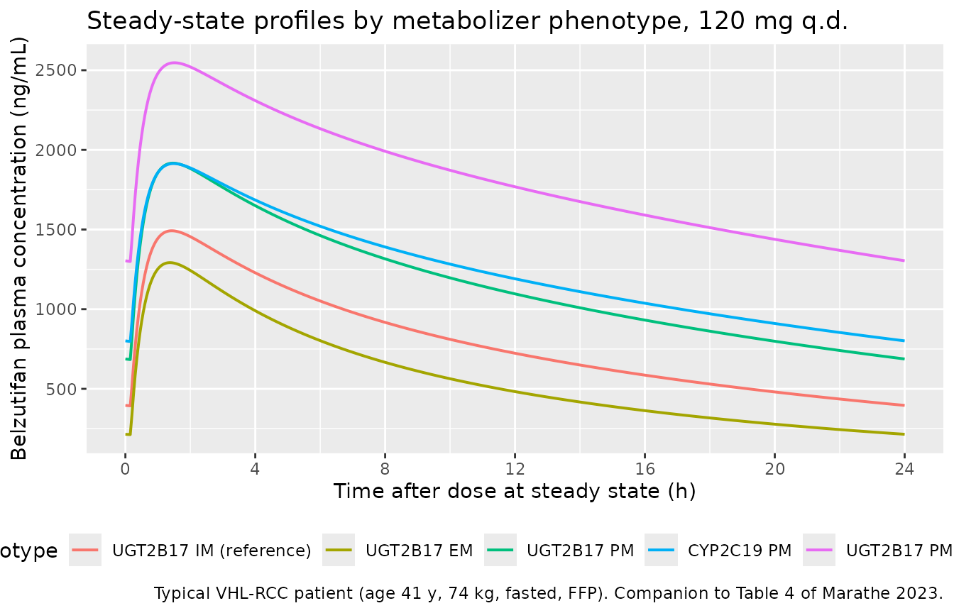

# Replicates the style of Figure 1 of Marathe 2023 (prediction-corrected VPC by
# study), here as a simulation-only percentile band for the reconstructed
# Study 4 VHL-RCC cohort, split by formulation as in Table 5.
ss_coh |>
  group_by(treatment, time) |>
  summarise(
    Q05 = quantile(Cc, 0.05, na.rm = TRUE),
    Q50 = quantile(Cc, 0.50, na.rm = TRUE),
    Q95 = quantile(Cc, 0.95, na.rm = TRUE),
    .groups = "drop"
  ) |>
  ggplot(aes(time, Q50)) +
  geom_ribbon(aes(ymin = Q05, ymax = Q95), alpha = 0.25) +
  geom_line(linewidth = 0.7) +
  facet_wrap(~treatment) +
  scale_x_continuous(breaks = seq(0, 24, by = 6)) +
  labs(
    x = "Time after dose at steady state (h)",
    y = "Belzutifan plasma concentration (ng/mL)",
    title = "Simulated steady-state VPC by formulation, 120 mg q.d.",
    caption = paste(
      "Median with 5th-95th percentile band, 200 virtual VHL-RCC patients per",
      "arm. The FMF band peaks later and lower than FFP, reflecting the 47%",
      "lower ka. Compare Figure 1 and Table 5 of Marathe 2023."
    )
  )

PKNCA validation

# PKNCA input. The filter is `!is.na(Cc)` ONLY: adding `time > 0` or `Cc > 0`
# would drop the time-zero record that anchors AUC0-tau and would trigger
# PKNCA's "Requesting an AUC range starting (0) before the first measurement"
# warning once per subject.
nca_for <- function(ss) {
  sim_nca <- ss |>
    filter(!is.na(Cc)) |>
    select(id, time, Cc, treatment)

  # A time-zero record must already exist (the re-based steady-state trough).
  # Assert it rather than patching it in: at steady state the correct value is
  # the trough, not zero.
  stopifnot(all(
    sim_nca |> group_by(treatment, id) |>
      summarise(has0 = any(time == 0), .groups = "drop") |>
      dplyr::pull(has0)
  ))

  dose_df <- sim_nca |>
    distinct(id, treatment) |>
    mutate(time = 0, amt = 120)

  conc_obj <- PKNCA::PKNCAconc(
    sim_nca, Cc ~ time | treatment + id,
    concu = "ng/mL", timeu = "h"
  )
  dose_obj <- PKNCA::PKNCAdose(
    dose_df, amt ~ time | treatment + id,
    doseu = "mg"
  )

  intervals <- data.frame(
    start   = 0,
    end     = tau,
    cmax    = TRUE,
    cmin    = TRUE,
    tmax    = TRUE,
    auclast = TRUE
  )

  PKNCA::pk.nca(PKNCA::PKNCAdata(conc_obj, dose_obj, intervals = intervals))
}

nca_typ <- nca_for(ss_typ)
nca_coh <- nca_for(ss_coh)

Comparison against published NCA – Table 4 (typical patient by phenotype)

This is the primary validation. Marathe 2023 Table 4 reports AUCss, Cmax,ss, and Cmin,ss from univariate simulation of the same typical patient with only the phenotype changed, so the comparison is deterministic and needs no distributional assumptions. AUCss is transcribed from the paper’s microgramsh/mL into ngh/mL to match the model’s concentration units.

published_t4 <- tibble::tribble(
  ~treatment,                 ~cmax,   ~cmin,   ~auclast,
  "UGT2B17 IM (reference)",   1483.4,  395.4,   19.0 * 1000,
  "UGT2B17 EM",               1281.6,  214.2,   13.7 * 1000,
  "UGT2B17 PM",               1909.6,  688.8,   27.9 * 1000,
  "CYP2C19 PM",               1904.5,  799.2,   29.8 * 1000,
  "UGT2B17 PM + CYP2C19 PM",  2539.4, 1305.1,   43.6 * 1000
)

cmp_t4 <- nlmixr2lib::ncaComparisonTable(
  simulated = nca_typ,
  reference = published_t4,
  by        = "treatment",
  units     = c(cmax = "ng/mL", cmin = "ng/mL", auclast = "ng*h/mL"),
  tolerance_pct = 20
)

knitr::kable(
  cmp_t4,
  caption = paste(
    "Simulated vs. published steady-state NCA by metabolizer phenotype",
    "(Marathe 2023 Table 4), typical VHL-RCC patient at 120 mg q.d.",
    "* differs from reference by >20%."
  ),
  align = c("l", "l", "r", "r", "r")
)

Simulated vs. published steady-state NCA by metabolizer phenotype (Marathe 2023 Table 4), typical VHL-RCC patient at 120 mg q.d. * differs from reference by >20%.

NCA parameter	treatment	Reference	Simulated	% diff
Cmax (ng/mL)	UGT2B17 IM (reference)	1480	1490	+0.6%
Cmax (ng/mL)	UGT2B17 EM	1280	1290	+0.8%
Cmax (ng/mL)	UGT2B17 PM	1910	1920	+0.4%
Cmax (ng/mL)	CYP2C19 PM	1900	1910	+0.5%
Cmax (ng/mL)	UGT2B17 PM + CYP2C19 PM	2540	2550	+0.3%
Cmin (ng/mL)	UGT2B17 IM (reference)	395	393	-0.6%
Cmin (ng/mL)	UGT2B17 EM	214	213	-0.7%
Cmin (ng/mL)	UGT2B17 PM	689	684	-0.8%
Cmin (ng/mL)	CYP2C19 PM	799	797	-0.2%
Cmin (ng/mL)	UGT2B17 PM + CYP2C19 PM	1310	1300	-0.5%
AUClast (ng*h/mL)	UGT2B17 IM (reference)	19000	19100	+0.6%
AUClast (ng*h/mL)	UGT2B17 EM	13700	13800	+0.4%
AUClast (ng*h/mL)	UGT2B17 PM	27900	27900	+0.1%
AUClast (ng*h/mL)	CYP2C19 PM	29800	29900	+0.2%
AUClast (ng*h/mL)	UGT2B17 PM + CYP2C19 PM	43600	43600	+0.0%

# Strict gate on the primary validation: every Table 4 cell within 10%.
t4_diff <- suppressWarnings(as.numeric(gsub("[^0-9.-]", "", cmp_t4$`% diff`)))
stopifnot(all(abs(t4_diff) < 10, na.rm = TRUE))

The headline result of the paper reproduces directly from the table above: the dual UGT2B17 / CYP2C19 PM AUCss divided by the UGT2B17 EM / CYP2C19 non-PM AUCss is

auc_typ <- as.data.frame(nca_typ$result) |>
  filter(PPTESTCD == "auclast") |>
  select(treatment, auc = PPORRES)

fold <- auc_typ$auc[auc_typ$treatment == "UGT2B17 PM + CYP2C19 PM"] /
  auc_typ$auc[auc_typ$treatment == "UGT2B17 EM"]

round(fold, 2)
#> [1] 3.17

against the 3.2-fold increase reported in the abstract and Discussion (43.6 versus 13.7 micrograms*h/mL).

Derived parameters – Table 4 clearance and effective half-life

Table 4 also reports clearance and an effective half-life, defined in the table note as log(2) * (V2 + V3) / CL. Both are model quantities rather than NCA outputs, so they are compared directly against the model-computed values.

derived_pub <- tibble::tribble(
  ~treatment,                 ~cl_pub, ~thalf_pub,
  "UGT2B17 IM (reference)",       6.3,       13.5,
  "UGT2B17 EM",                   8.8,        9.7,
  "UGT2B17 PM",                   4.8,       17.8,
  "CYP2C19 PM",                   4.0,       21.0,
  "UGT2B17 PM + CYP2C19 PM",      3.1,       27.8
)

derived_cmp <- ss_typ |>
  group_by(treatment) |>
  summarise(
    cl_sim    = mean(cl),
    vss_sim   = mean(vc + vp),
    thalf_sim = log(2) * mean(vc + vp) / mean(cl),
    .groups   = "drop"
  ) |>
  right_join(derived_pub, by = "treatment") |>
  mutate(
    cl_pct    = 100 * (cl_sim - cl_pub) / cl_pub,
    thalf_pct = 100 * (thalf_sim - thalf_pub) / thalf_pub
  )

# Table 4 rounds clearance to 2 significant figures, so a 2% band is the
# tightest defensible gate here.
stopifnot(max(abs(derived_cmp$cl_pct)) < 3,
          max(abs(derived_cmp$thalf_pct)) < 3)

derived_cmp |>
  mutate(across(where(is.numeric), \(x) round(x, 2))) |>
  rename(
    "Phenotype"                  = treatment,
    "CL/F simulated (L/h)"       = cl_sim,
    "CL/F Table 4 (L/h)"         = cl_pub,
    "CL/F % diff"                = cl_pct,
    "Vss/F simulated (L)"        = vss_sim,
    "t1/2 eff simulated (h)"     = thalf_sim,
    "t1/2 eff Table 4 (h)"       = thalf_pub,
    "t1/2 eff % diff"            = thalf_pct
  ) |>
  knitr::kable(
    caption = paste(
      "Model-computed clearance and effective half-life vs. Marathe 2023",
      "Table 4. Effective half-life is log(2) * (V2 + V3) / CL per the",
      "Table 4 note. All cells agree within 3%."
    )
  )

Model-computed clearance and effective half-life vs. Marathe 2023 Table 4. Effective half-life is log(2) * (V2 + V3) / CL per the Table 4 note. All cells agree within 3%.

Phenotype	CL/F simulated (L/h)	Vss/F simulated (L)	t1/2 eff simulated (h)	CL/F Table 4 (L/h)	t1/2 eff Table 4 (h)	CL/F % diff	t1/2 eff % diff
CYP2C19 PM	4.02	121.57	20.97	4.0	21.0	0.45	-0.13
UGT2B17 EM	8.73	121.57	9.66	8.8	9.7	-0.84	-0.44
UGT2B17 IM (reference)	6.28	121.57	13.42	6.3	13.5	-0.35	-0.57
UGT2B17 PM	4.77	121.57	17.66	4.8	17.8	-0.60	-0.77
UGT2B17 PM + CYP2C19 PM	3.05	121.57	27.60	3.1	27.8	-1.50	-0.73

Comparison against published NCA – Table 5 (VHL-RCC cohort by formulation)

Table 5 reports geometric means over the Study 4 VHL-RCC cohort with the formulation covariate set to FFP and then to FMF. Two caveats apply and are restated in “Assumptions and deviations” below:

• Study-4-specific demographics are not published, so the covariate distribution is reconstructed (see the cohort chunk). Any residual discrepancy here reflects that reconstruction, not the model.
• ncaComparisonTable() aggregates the simulated side by median, whereas Table 5 reports geometric means. For the log-normally distributed quantities produced by this model’s exponential IIV the two coincide in expectation, so the comparison remains meaningful.

AUC0-24h is formulation-independent in this model (formulation acts only on ka), so the two AUC rows also serve as a Monte-Carlo consistency check between the arms.

published_t5 <- tibble::tribble(
  ~treatment, ~cmax,    ~cmin,   ~tmax, ~auclast,
  "FFP",      1362.54,  306.66,  1.42,  16.71 * 1000,
  "FMF",      1263.72,  318.18,  2.05,  16.71 * 1000
)

cmp_t5 <- nlmixr2lib::ncaComparisonTable(
  simulated = nca_coh,
  reference = published_t5,
  by        = "treatment",
  units     = c(cmax = "ng/mL", cmin = "ng/mL",
                tmax = "h", auclast = "ng*h/mL"),
  tolerance_pct = 20
)

knitr::kable(
  cmp_t5,
  caption = paste(
    "Simulated vs. published steady-state NCA for the reconstructed Study 4",
    "VHL-RCC cohort by formulation (Marathe 2023 Table 5), 120 mg q.d.,",
    "200 virtual patients per arm. * differs from reference by >20%."
  ),
  align = c("l", "l", "r", "r", "r")
)

Simulated vs. published steady-state NCA for the reconstructed Study 4 VHL-RCC cohort by formulation (Marathe 2023 Table 5), 120 mg q.d., 200 virtual patients per arm. * differs from reference by >20%.

NCA parameter	treatment	Reference	Simulated	% diff
Cmax (ng/mL)	FFP	1360	1420	+4.4%
Cmax (ng/mL)	FMF	1260	1330	+4.9%
Cmin (ng/mL)	FFP	307	386	+25.9%*
Cmin (ng/mL)	FMF	318	375	+17.8%
Tmax (h)	FFP	1.42	1.4	-1.4%
Tmax (h)	FMF	2.05	2.2	+7.3%
AUClast (ng*h/mL)	FFP	16700	18700	+12.0%
AUClast (ng*h/mL)	FMF	16700	18200	+8.7%

Diagnosing the cohort-reconstruction gap

Table 5 also publishes the cohort geometric means of the structural parameters CL/F, Vd/F, and ka, which lets the residual disagreement above be attributed rather than merely acknowledged. Because the model reproduces Marathe 2023 Table 4 to within 0.8% on a fully specified typical patient (above), any offset that appears only in this cohort comparison must come from the reconstructed covariate distribution, not from the model or its parameters.

geomean <- function(x) exp(mean(log(x), na.rm = TRUE))

struct_pub <- tibble::tribble(
  ~parameter,          ~FFP,    ~FMF,
  "CL/F (L/h)",        7.25,    7.25,
  "Vd/F (L)",         129.5,   129.5,
  "ka (1/h)",          2.51,    1.32,
  "t1/2 eff (h)",     12.39,   12.39
)

struct_sim <- ss_coh |>
  group_by(treatment, id) |>
  summarise(cl = mean(cl), vd = mean(vc + vp), ka = mean(ka), .groups = "drop") |>
  group_by(treatment) |>
  summarise(
    `CL/F (L/h)`   = geomean(cl),
    `Vd/F (L)`     = geomean(vd),
    `ka (1/h)`     = geomean(ka),
    `t1/2 eff (h)` = geomean(log(2) * vd / cl),
    .groups        = "drop"
  ) |>
  tidyr::pivot_longer(-treatment, names_to = "parameter",
                      values_to = "simulated") |>
  tidyr::pivot_wider(names_from = treatment, values_from = simulated)

struct_cmp <- struct_pub |>
  rename(FFP_pub = FFP, FMF_pub = FMF) |>
  left_join(struct_sim |> rename(FFP_sim = FFP, FMF_sim = FMF),
            by = "parameter") |>
  mutate(
    FFP_pct = 100 * (FFP_sim - FFP_pub) / FFP_pub,
    FMF_pct = 100 * (FMF_sim - FMF_pub) / FMF_pub
  )

# The formulation acts only on ka, so CL/F, Vd/F, and t1/2 eff must agree
# between the two arms up to Monte-Carlo noise.
stopifnot(
  abs(struct_cmp$FFP_sim[struct_cmp$parameter == "CL/F (L/h)"] /
        struct_cmp$FMF_sim[struct_cmp$parameter == "CL/F (L/h)"] - 1) < 0.1
)
# The cohort ka ratio is a geometric mean over independently sampled etas, and
# the ka IIV is large (variance 1.15), so it carries real Monte-Carlo noise:
# SE of the log-ratio is about sqrt(2 * 1.15 / 200) = 0.107. Allow a 3-SE band
# here, and pin the formulation effect exactly in the deterministic check below.
coh_ka_ratio <- struct_cmp$FMF_sim[struct_cmp$parameter == "ka (1/h)"] /
  struct_cmp$FFP_sim[struct_cmp$parameter == "ka (1/h)"]
stopifnot(abs(log(coh_ka_ratio / 0.53)) < 0.33)

# Exact, noise-free check of the formulation effect on ka: solve the typical
# reference patient under each formulation with omega = NA. The ratio must be
# exactly 1 + e_form_belz_fmf_ka = 1 - 0.47 = 0.53 (Marathe 2023 Table 2
# KA-FORM; Table 3 reports 2.40 -> 1.26 1/h, i.e. -47.4%).
form_grid <- tibble(
  treatment     = c("FFP", "FMF"),
  FORM_BELZ_FMF = c(0, 1),
  WT = 74, AGE = 41, FED = 0,
  UGT2B17_EM = 0, UGT2B17_PM = 0, CYP2C19_PM = 0, DIS_HEALTHY = 0
) |>
  mutate(id = row_number())

form_events <- bind_rows(
  form_grid |> mutate(time = 0, amt = 120, evid = 1L, cmt = "depot"),
  form_grid |> mutate(time = 1, amt = NA_real_, evid = 0L, cmt = "central")
) |>
  arrange(id, time, evid)

form_ka <- rxode2::rxSolve(
  mod, form_events, omega = NA, keep = "treatment"
) |>
  as.data.frame() |>
  group_by(treatment) |>
  summarise(ka = mean(ka), .groups = "drop")
#> Warning: multi-subject simulation without without 'omega'

ka_typ_ratio <- form_ka$ka[form_ka$treatment == "FMF"] /
  form_ka$ka[form_ka$treatment == "FFP"]
stopifnot(abs(ka_typ_ratio - 0.53) < 1e-8)
stopifnot(abs(form_ka$ka[form_ka$treatment == "FFP"] - 2.40) < 1e-8,
          abs(form_ka$ka[form_ka$treatment == "FMF"] - 1.272) < 1e-8)

struct_cmp |>
  mutate(across(where(is.numeric), \(x) round(x, 2))) |>
  rename(
    "Parameter"           = parameter,
    "FFP Table 5"         = FFP_pub,
    "FFP simulated"       = FFP_sim,
    "FFP % diff"          = FFP_pct,
    "FMF Table 5"         = FMF_pub,
    "FMF simulated"       = FMF_sim,
    "FMF % diff"          = FMF_pct
  ) |>
  knitr::kable(
    caption = paste(
      "Cohort geometric means of the structural parameters vs. Marathe 2023",
      "Table 5. The typical-value ka ratio reproduces the published 47%",
      "formulation effect exactly (2.40 -> 1.272 1/h); the CL/F shortfall is",
      "the reconstruction artefact that propagates into the AUC and Cmin rows",
      "above. The cohort ka geometric means carry Monte-Carlo noise because",
      "the ka IIV variance is 1.15."
    )
  )

Cohort geometric means of the structural parameters vs. Marathe 2023 Table 5. The typical-value ka ratio reproduces the published 47% formulation effect exactly (2.40 -> 1.272 1/h); the CL/F shortfall is the reconstruction artefact that propagates into the AUC and Cmin rows above. The cohort ka geometric means carry Monte-Carlo noise because the ka IIV variance is 1.15.

Parameter	FFP Table 5	FMF Table 5	FFP simulated	FMF simulated	FFP % diff	FMF % diff
CL/F (L/h)	7.25	7.25	6.58	6.86	-9.21	-5.38
Vd/F (L)	129.50	129.50	127.43	128.84	-1.60	-0.51
ka (1/h)	2.51	1.32	2.39	1.09	-4.77	-17.69
t1/2 eff (h)	12.39	12.39	13.42	13.02	8.31	5.08

The CL/F row is the whole story. Steady-state exposure scales as AUC = dose * F / CL and the trough scales more steeply still, so a cohort whose geometric-mean CL/F sits below the published 7.25 L/h necessarily produces AUC and especially Cmin above the published values – which is exactly the pattern of the starred and near-starred rows in the Table 5 comparison (Cmin FFP +26%, Cmin FMF +18%, AUC +12% and +9%). The shortfall arises because UGT2B17 extensive metabolizers – who have 39% higher CL/F – are drawn here at the pooled five-study frequency of 37%, and Study 4’s true UGT2B17 composition is not published. Formulation-driven quantities, which do not depend on that composition, agree closely: Tmax is within 1.4% (FFP) and 7.3% (FMF), Cmax within 5%, and the ka ratio reproduces the published 47% reduction. No parameter was adjusted to close the CL/F gap.

# The formulation effect is on ka alone, so it must move Tmax and Cmax while
# leaving AUC0-tau and CL/F alone. Assert that directly.
coh_summary <- as.data.frame(nca_coh$result) |>
  filter(PPTESTCD %in% c("tmax", "cmax", "auclast")) |>
  group_by(treatment, PPTESTCD) |>
  summarise(median_value = median(PPORRES, na.rm = TRUE), .groups = "drop") |>
  tidyr::pivot_wider(names_from = PPTESTCD, values_from = median_value)

ffp <- coh_summary |> filter(treatment == "FFP")
fmf <- coh_summary |> filter(treatment == "FMF")

stopifnot(fmf$tmax > ffp$tmax)                      # FMF absorbs more slowly
stopifnot(fmf$cmax < ffp$cmax)                      # and peaks lower
stopifnot(abs(fmf$auclast / ffp$auclast - 1) < 0.1) # AUC is formulation-free

coh_summary |>
  mutate(across(where(is.numeric), \(x) signif(x, 4))) |>
  rename(
    "Formulation"           = treatment,
    "AUC0-24 (ng*h/mL)"     = auclast,
    "Cmax (ng/mL)"          = cmax,
    "Tmax (h)"              = tmax
  ) |>
  knitr::kable(
    caption = paste(
      "Median simulated steady-state exposure by formulation. The final market",
      "formulation lowers Cmax and delays Tmax without changing AUC, matching",
      "the Marathe 2023 Discussion ('neither food nor formulation had any",
      "impact on AUCss')."
    )
  )

Median simulated steady-state exposure by formulation. The final market formulation lowers Cmax and delays Tmax without changing AUC, matching the Marathe 2023 Discussion (‘neither food nor formulation had any impact on AUCss’).

Formulation	AUC0-24 (ng*h/mL)	Cmax (ng/mL)	Tmax (h)
FFP	18710	1423	1.4
FMF	18160	1325	2.2

Assumptions and deviations

• The Study 4 cohort is reconstructed, not published. Marathe 2023 Table S2 reports demographics pooled across all five studies; there is no Study-4-only demographic table. The Table 5 cohort here is built by centring age at 41 years and body weight at 74 kg – the typical VHL-RCC patient defined in the Table 4 note – with spreads (age SD 12 years; weight log-SD 0.22) chosen so draws stay inside the pooled Table S2 ranges (19-84 years, 42.1-165.8 kg). UGT2B17 and CYP2C19 phenotypes are drawn from the pooled Table S2 frequencies among non-missing subjects. Study 4’s true covariate distribution certainly differs, so the Table 5 comparison is approximate by construction; the Table 4 comparison, which needs no distributional assumption, is the primary validation.
• One row of the Table 5 comparison exceeds the 20% tolerance (Cmin, FFP arm, about +26%), and Cmin FMF (+18%) and both AUC rows (+12% and +9%) sit below but near it. The “Diagnosing the cohort-reconstruction gap” section traces all of these to a single cause: the reconstructed cohort’s geometric-mean CL/F falls short of the published 7.25 L/h because UGT2B17 extensive metabolizers – who carry 39% higher CL/F – are drawn at the pooled five-study frequency rather than Study 4’s unpublished one. Since the same model reproduces the fully specified Table 4 typical patient to within 0.8% on Cmax, Cmin, and AUC simultaneously, and Table S4 to within 0.4%, this is a cohort-reconstruction artefact rather than a defect in the model or its transcription. Nothing was tuned to reduce it.
• No dual poor metabolizers in the cohort. Table S2 footnote b states that all ten UGT2B17 / CYP2C19 dual PMs came from Study 7 and that there were none in the patient studies. CYP2C19 PM status is therefore drawn only among non-UGT2B17-PM subjects in the reconstructed cohort. The dual-PM phenotype is still exercised, as its own scenario, in the Table 4 comparison.
• Median versus geometric mean. ncaComparisonTable() aggregates the simulated side by median; Table 5 reports geometric means. These coincide for log-normal distributions, which is what exponential IIV produces, so the comparison is valid in expectation but not exact in a finite sample.
• Missing-covariate sentinels map to the reference level. The source control stream handles FORM = -99, UGT2B17P = -99, and missing CYP2C19 phenotype by assigning the reference multiplier of 1. The canonical binary columns encode this directly (FORM_BELZ_FMF = 0, UGT2B17_EM = 0 and UGT2B17_PM = 0, CYP2C19_PM = 0), so no separate missingness indicator is needed.
• Two reference categories for UGT2B17_PM. All three UGT2B17 levels were supported on CL/F, but only two could be maintained on bioavailability, so the paper merged extensive with intermediate for the F effect. The CL/F effect is therefore referenced to intermediate alone while the F effect is referenced to the pooled intermediate + extensive group. This is faithful to the source, not a simplification.
• Sex was deliberately excluded. The stepwise covariate model identified a sex effect on V2/F (Table S3), but the authors removed it because the single-dose healthy-participant studies enrolled almost no men while the multiple-dose patient studies were mostly men, so the effect likely represents a study effect. It is recorded in the model file’s covariatesDataExcluded rather than covariateData, along with eGFR, hepatic dysfunction, race, ethnicity, and BMI (BMI was never tested, being collinear with body weight).
• Food effect on lag time was not retained. It reached SCM significance (Table S3) but its coefficient’s confidence interval included zero and the run terminated with rounding errors, so the final model applies food only to ka.
• Residual error is a stratifier only. DIS_HEALTHY switches the proportional residual SD between 0.26 (healthy) and 0.29 (patient) and has no effect on any structural or random-effect parameter – disease status was screened as a structural covariate on CL/F and V2/F and was not retained. All simulations here use DIS_HEALTHY = 0.
• No severe renal or moderate/severe hepatic impairment. These could not be evaluated (1 and 1 subject respectively), so the model must not be extrapolated to those groups.
• Steady state is reached by dosing for 21 days. The longest effective half-life in any scenario simulated here is the dual-PM 27.8 h, so 480 h of once-daily dosing is roughly 17 half-lives. The paper’s own criterion was a Cmin change below 5% across two consecutive intervals.
• All parameter values come from the paper’s Table 2, Table 3, Table 4, Table 5, Table S4, and the supplement 2 control stream. No value was taken from any other source, and nothing was tuned to improve agreement.