Axitinib (Garrett 2014)
Source:vignettes/articles/Garrett_2014_axitinib.Rmd
Garrett_2014_axitinib.RmdModel and source
- Citation: Garrett M, Poland B, Brennan M, Hee B, Pithavala YK, Amantea MA. Population pharmacokinetic analysis of axitinib in healthy volunteers. Br J Clin Pharmacol. 2014;77(3):480-492. doi:10.1111/bcp.12206
- Description: Two-compartment population PK model for axitinib in healthy volunteers (Garrett 2014). First-order absorption with fixed lag time, allometric power-form effect of body weight on the central volume of distribution (reference 75 kg), linear-proportional fasting effects on the first-order absorption rate constant ka and on bioavailability F, and a linear-proportional reduction in F for the marketed crystal polymorph Form XLI relative to the earlier Form IV reference. Pooled data from 337 healthy subjects across ten Pfizer Phase I studies.
- Article: https://doi.org/10.1111/bcp.12206
Garrett 2014 pooled plasma axitinib concentrations from 337 healthy
volunteers across ten Pfizer Phase I studies (Table 1) and fit a single
two-compartment population PK model with first-order absorption and a
fixed lag time. The food / formulation effects of clinical interest –
fasting on first-order absorption rate ka and on absolute
oral bioavailability F, plus the F reduction for the
marketed crystal polymorph Form XLI relative to the earlier Form IV
polymorph – were included in the base model and retained through the
formal covariate search (Methods ‘Model development’ and ‘Statistical
analysis’). Among the eleven additional covariates tested (body weight,
age, sex, race, smoking status, creatinine clearance, ALT, AST,
bilirubin, the UGT1A1*28 genotype, and the
CYP2C19 inferred phenotype), only the power-form effect of
body weight on the central volume Vc reached
formal-selection significance.
Population
The pooled dataset (Garrett 2014 Table 2; reproduced programmatically
via readModelDb("Garrett_2014_axitinib")$population) is
dominated by young (median 31 years), White (62%), male (93%),
non-smoking (88%) healthy volunteers with normal kidney and liver
function as evidenced by group-mean creatinine clearance 117.2 mL/min,
AST 23.9 U/L, ALT 24.1 U/L, and total bilirubin 0.8 mg/dL. Median total
body weight is 75.0 kg. Race distribution is White 62%, Black 8%, Asian
18%, Japanese 6%, Hispanic 3%, Other 3%. Genotyping for
UGT1A1*28 and the CYP2C19
*2 / *3 / *17 alleles was performed on the majority of
subjects; the bulk of the cohort is UGT1A1
TA6/TA6 (51%) and CYP2C19 extensive
metaboliser (93%). All studies enrolled in the United States, Belgium,
or Singapore; ten clinical sites are listed in the Methods ‘Study
design’ section. Pre-dose to 48 h dense sampling was performed in most
studies (per-study schedules in Table 1).
Source trace
The per-parameter origin is recorded as an in-file comment next to
each ini() entry in
inst/modeldb/specificDrugs/Garrett_2014_axitinib.R. The
table below collects them in one place for review.
| Equation / parameter | Value | Source location |
|---|---|---|
| Structural model – two-compartment with first-order absorption and lag time | n/a | Methods ‘Model development’; Results ‘PK base model’ |
| Reference body weight for allometric Vc | 75 kg | Results ‘Full model and final model’; Table 3 footnote (population median) |
lka (Form IV, fed reference) |
log(0.523) | Table 3 ‘k a (h-1) Form IV, Fed’ = 0.523 |
lcl |
log(17.0) | Table 3 ‘CL (L/h)’ final = 17.0 |
lvc (at 75 kg) |
log(45.3) | Table 3 ‘Vc (L)’ final = 45.3 |
lq |
log(1.74) | Table 3 ‘Q (L/h)’ final = 1.74 |
lvp |
log(45.9) | Table 3 ‘Vp (L)’ final = 45.9 |
lfdepot (Form IV, fed reference) |
log(0.465) | Table 3 ‘F, Form IV, Fed’ = 0.465 |
ltlag (FIXED) |
log(0.457) | Table 3 ‘tlag (h)’ = 0.457 (Table 3 footnote: fixed at 0.457 in the final run) |
e_wt_vc (allometric Vc exponent) |
0.758 | Table 3 ‘Weight effect on Vc’ = 0.758 |
e_fast_ka (fasting on ka) |
2.07 | Table 3 ‘ka Fasting’ = 2.07 |
e_fast_f (fasting on F) |
0.338 | Table 3 ‘F Fasting’ = 0.338 |
e_xli_f (Form XLI on F) |
-0.150 | Table 3 ‘F Form XLI’ = -0.150 |
omega^2 CL, cov(CL,Vc),
omega^2 Vc
|
0.272, 0.141, 0.0949 | Table 3 (block) |
omega^2 Q, cov(Q,Vp),
omega^2 Vp
|
0.406, 0.619, 1.07 | Table 3 (block) |
omega^2 ka |
0.506 | Table 3 final |
expSd (oral log-additive residual SD) |
0.509 | Table 3 ‘Oral, %’ final = 50.9% |
| IV log-additive residual SD (not encoded) | 0.342 | Table 3 ‘Intravenous, %’ final = 34.2% (see Assumptions below) |
Virtual cohort
Original observed data are not publicly available. The simulation cohorts below approximate the published Phase I trial demographics (Garrett 2014 Table 2): a healthy-adult cohort with body weight distributed around the population median 75 kg.
set.seed(20140311)

n_per_arm <- 100L

make_cohort <- function(n, fed_value, form_xli_value, label, id_offset = 0L) {
  wt <- pmax(50, rnorm(n, mean = 75, sd = 11.6))
  dosing <- tibble::tibble(
    id   = id_offset + seq_len(n),
    time = 0,
    evid = 1L,
    amt  = 5,                                # 5 mg oral axitinib (Garrett 2014 Methods Table 1)
    cmt  = "depot",
    WT   = wt,
    FED  = fed_value,
    FORM_AXI_XLI = form_xli_value,
    treatment    = label
  )
  obs_times <- c(0.5, 1, 1.5, 2, 3, 4, 6, 8, 12, 16, 24, 32, 36, 48)
  obs <- tidyr::expand_grid(
    id   = id_offset + seq_len(n),
    time = obs_times
  ) |>
    dplyr::left_join(
      dosing |> dplyr::select(id, WT, FED, FORM_AXI_XLI, treatment),
      by = "id"
    ) |>
    dplyr::mutate(evid = 0L, amt = 0, cmt = "central")
  dplyr::bind_rows(dosing, obs) |> dplyr::arrange(id, time, dplyr::desc(evid))
}

events <- dplyr::bind_rows(
  make_cohort(n_per_arm, fed_value = 1L, form_xli_value = 0L, label = "Form IV fed",     id_offset = 0L),
  make_cohort(n_per_arm, fed_value = 0L, form_xli_value = 0L, label = "Form IV fasted",  id_offset =  n_per_arm),
  make_cohort(n_per_arm, fed_value = 1L, form_xli_value = 1L, label = "Form XLI fed",    id_offset = 2L * n_per_arm)
)

stopifnot(!anyDuplicated(unique(events[, c("id", "time", "evid")])))
Simulation
mod <- readModelDb("Garrett_2014_axitinib")

sim <- rxode2::rxSolve(
  mod,
  events = as.data.frame(events),
  keep   = c("treatment", "WT", "FED", "FORM_AXI_XLI"),
  nStud  = 1L
) |>
  as.data.frame() |>
  dplyr::mutate(treatment = factor(treatment, levels = c("Form IV fed", "Form IV fasted", "Form XLI fed")))
#> ℹ parameter labels from comments will be replaced by 'label()'
Replicate published figures
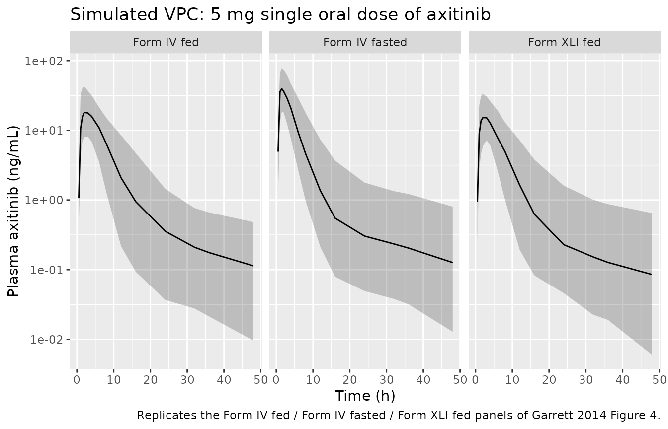
Garrett 2014 Figure 4 shows visual predictive checks of the final model against pooled observed data from four of the ten studies (study 1 Form IV fasted; study 2 Form IV fed and fasted; study 6 Form IV fasted; study 7 Form IV vs Form XLI both fed). Observed data are not publicly distributed, so the panel below reproduces the simulated median and 90% prediction interval from the packaged model under the three formulation x food conditions Garrett 2014 emphasises.
sim |>
  dplyr::filter(time > 0) |>
  dplyr::group_by(treatment, time) |>
  dplyr::summarise(
    Q05 = stats::quantile(Cc, 0.05, na.rm = TRUE),
    Q50 = stats::quantile(Cc, 0.50, na.rm = TRUE),
    Q95 = stats::quantile(Cc, 0.95, na.rm = TRUE),
    .groups = "drop"
  ) |>
  ggplot(aes(time, Q50)) +
  geom_ribbon(aes(ymin = Q05, ymax = Q95), alpha = 0.25) +
  geom_line() +
  facet_wrap(~ treatment) +
  scale_y_log10() +
  labs(
    x = "Time (h)",
    y = "Plasma axitinib (ng/mL)",
    title = "Simulated VPC: 5 mg single oral dose of axitinib",
    caption = "Replicates the Form IV fed / Form IV fasted / Form XLI fed panels of Garrett 2014 Figure 4."
  )
PKNCA validation
Single-dose NCA over the 0-48 h sampling window, stratified by
formulation x food state. The grouping variable treatment
matches the cohort labels carried through
rxSolve(..., keep = ).
sim_nca <- sim |>
  dplyr::filter(!is.na(Cc)) |>
  dplyr::select(id, time, Cc, treatment)

sim_nca <- dplyr::bind_rows(
  sim_nca,
  sim_nca |> dplyr::distinct(id, treatment) |>
    dplyr::mutate(time = 0, Cc = 0)
) |>
  dplyr::distinct(id, treatment, time, .keep_all = TRUE) |>
  dplyr::arrange(id, treatment, time)

dose_df <- events |>
  dplyr::filter(evid == 1L) |>
  dplyr::select(id, time, amt, treatment) |>
  as.data.frame()

conc_obj <- PKNCA::PKNCAconc(
  as.data.frame(sim_nca),
  Cc ~ time | treatment + id,
  concu = "ng/mL",
  timeu = "h"
)

dose_obj <- PKNCA::PKNCAdose(
  dose_df,
  amt ~ time | treatment + id,
  doseu = "mg"
)

intervals <- data.frame(
  start       = 0,
  end         = Inf,
  cmax        = TRUE,
  tmax        = TRUE,
  aucinf.obs  = TRUE,
  half.life   = TRUE
)

nca_res <- PKNCA::pk.nca(PKNCA::PKNCAdata(conc_obj, dose_obj, intervals = intervals))

nca_summary <- as.data.frame(nca_res$result) |>
  dplyr::filter(PPTESTCD %in% c("cmax", "tmax", "aucinf.obs", "half.life")) |>
  dplyr::group_by(treatment, PPTESTCD) |>
  dplyr::summarise(median_value = stats::median(PPORRES, na.rm = TRUE), .groups = "drop") |>
  tidyr::pivot_wider(names_from = PPTESTCD, values_from = median_value)

knitr::kable(
  nca_summary,
  digits  = 3,
  caption = "Simulated single-dose median NCA parameters by formulation x food state."
)| treatment | aucinf.obs | cmax | half.life | tmax |
|---|---|---|---|---|
| Form IV fasted | 174.644 | 41.883 | 21.714 | 1.5 |
| Form IV fed | 141.330 | 18.779 | 19.366 | 3.0 |
| Form XLI fed | 106.399 | 16.311 | 18.268 | 3.0 |
Comparison against published structural effects
Garrett 2014 does not tabulate single-dose NCA values directly, but
the ratios between the three arms are completely determined by the Table
3 fasting and formulation effects on ka and
F:
-
AUC(Form IV fasted) / AUC(Form IV fed) = 1 + 0.338 = 1.338(fasting increases F by 33.8%;kadoes not enter the AUC ratio because CL, Vc, Q, and Vp are unchanged). -
AUC(Form XLI fed) / AUC(Form IV fed) = 1 - 0.150 = 0.850(Form XLI reduces F by 15%). -
Cmax(Form IV fasted) / Cmax(Form IV fed)increases with both the higher F and the 207%-higherka(faster absorption shifts the peak earlier and higher).
ratio_table <- nca_summary |>
  dplyr::select(treatment, aucinf.obs) |>
  tibble::deframe()

paper_auc_ratios <- tibble::tibble(
  ratio                     = c("Form IV fasted / Form IV fed", "Form XLI fed / Form IV fed"),
  simulated_AUC_ratio       = c(
    unname(ratio_table["Form IV fasted"] / ratio_table["Form IV fed"]),
    unname(ratio_table["Form XLI fed"]   / ratio_table["Form IV fed"])
  ),
  published_AUC_ratio_from_Table3 = c(1 + 0.338, 1 - 0.150)
)

knitr::kable(
  paper_auc_ratios,
  digits = 3,
  caption = "Simulated AUC(0-Inf) ratios vs published F-effect ratios (Garrett 2014 Table 3)."
)| ratio | simulated_AUC_ratio | published_AUC_ratio_from_Table3 |
|---|---|---|
| Form IV fasted / Form IV fed | 1.236 | 1.338 |
| Form XLI fed / Form IV fed | 0.753 | 0.850 |
Body-weight body-Cmax simulation (Garrett 2014 Results section)
Garrett 2014 separately reports a typical-value simulation of steady-state Cmax for the marketed 5 mg BID Form XLI fed regimen at three body-weight strata (Results ‘Full model and final model’): the 10th-percentile 62 kg subject (20.6 ng/mL), the median 75 kg subject (19.3 ng/mL), and the 90th-percentile 93 kg subject (17.9 ng/mL). The following block reproduces those Cmax values with a deterministic typical-value simulation (random effects zeroed).
mod_typ <- rxode2::zeroRe(mod)
#> ℹ parameter labels from comments will be replaced by 'label()'

ss_cohort <- function(weight_kg, label) {
  doses <- tibble::tibble(
    id   = 1L,
    time = seq(0, 24 * 14, by = 12),    # 5 mg BID for two weeks (more than enough to reach steady state)
    evid = 1L,
    amt  = 5,
    cmt  = "depot",
    WT   = weight_kg,
    FED  = 1L,
    FORM_AXI_XLI = 1L,
    treatment    = label
  )
  obs <- tibble::tibble(
    id   = 1L,
    time = seq(0, 24 * 14 + 12, by = 0.5),
    evid = 0L,
    amt  = 0,
    cmt  = "central",
    WT   = weight_kg,
    FED  = 1L,
    FORM_AXI_XLI = 1L,
    treatment    = label
  )
  dplyr::bind_rows(doses, obs) |> dplyr::arrange(time, dplyr::desc(evid))
}

ss_events <- dplyr::bind_rows(
  ss_cohort(62, "62 kg (10th pctile)") |> dplyr::mutate(id = 1L),
  ss_cohort(75, "75 kg (median)")      |> dplyr::mutate(id = 2L),
  ss_cohort(93, "93 kg (90th pctile)") |> dplyr::mutate(id = 3L)
)

ss_sim <- rxode2::rxSolve(
  mod_typ,
  events = as.data.frame(ss_events),
  keep   = c("treatment", "WT")
) |>
  as.data.frame()
#> ℹ omega/sigma items treated as zero: 'etalcl', 'etalvc', 'etalq', 'etalvp', 'etalka'
#> Warning: multi-subject simulation without without 'omega'

tau          <- 12
last_dose    <- max(ss_events$time[ss_events$evid == 1L])
ss_window_lo <- last_dose
ss_window_hi <- last_dose + tau

ss_cmax_sim <- ss_sim |>
  dplyr::filter(time >= ss_window_lo, time <= ss_window_hi) |>
  dplyr::group_by(treatment) |>
  dplyr::summarise(cmax_ss_sim = max(Cc), .groups = "drop")

ss_cmax_published <- tibble::tibble(
  treatment           = c("62 kg (10th pctile)", "75 kg (median)", "93 kg (90th pctile)"),
  cmax_ss_published   = c(20.6, 19.3, 17.9)
)

ss_cmax_compare <- dplyr::left_join(ss_cmax_sim, ss_cmax_published, by = "treatment") |>
  dplyr::mutate(pct_diff = 100 * (cmax_ss_sim - cmax_ss_published) / cmax_ss_published)

knitr::kable(
  ss_cmax_compare,
  digits  = 2,
  caption = "Simulated vs Garrett 2014 published typical-value steady-state Cmax for 5 mg BID Form XLI fed axitinib (ng/mL) at three body weights."
)| treatment | cmax_ss_sim | cmax_ss_published | pct_diff |
|---|---|---|---|
| 62 kg (10th pctile) | 20.57 | 20.6 | -0.14 |
| 75 kg (median) | 19.30 | 19.3 | 0.01 |
| 93 kg (90th pctile) | 17.91 | 17.9 | 0.08 |
Assumptions and deviations
-
Route-stratified residual error not encoded.
Garrett 2014 fit two log-additive residual SDs – oral 50.9% and
intravenous 34.2% (Table 3 final). The packaged model encodes a single
expSd = 0.509(the oral residual) because the model is intended for simulating oral dosing of the marketed axitinib tablet; the 16 IV-arm subjects from study 3 contributed primarily to the absolute-bioavailability anchor and are not the typical-use case. Users who need to simulate the IV arm at its reported residual variability should overrideexpSd <- 0.342afterreadModelDb(). -
Cohort body-weight distribution truncated at 50 kg.
The Phase I virtual cohort draws weights from
Normal(mean = 75, SD = 11.6)matched to Garrett 2014 Table 2 but truncated below at 50 kg so the simulated lighter-end weights remain consistent with the actual Phase I enrolment ceiling on lower body weight (no observed subjects below approximately 50 kg). The truncation has no effect on the Form XLI body-weight Cmax replication (62 / 75 / 93 kg are all well above the 50 kg floor). - Race / sex / smoking / genotype distributions are not simulated. Garrett 2014 found none of these covariates significant on CL or Vc in the final model (Results ‘Full model and final model’), so the packaged virtual cohort omits them. Users who want to simulate specific subgroups can pass additional columns through the event table, but the model itself ignores them.
-
tlagfixed at 0.457 h. The Table 3 footnote (double-dagger) notes that the final-model run reported in Table 3 was rerun withtlagfixed at 0.457 h to obtain a successful covariance step; estimates with fixedtlagmatched the free-tlagrun or differed by no more than 2 in the last significant digit. The packaged model encodestlagas fixed accordingly. -
FED covariate sense. The packaged model uses
FED = 1for the fed state (the reference category matching Garrett 2014 Table 3’s ‘Form IV, Fed’ typical values). The fasting effect is activated byFED = 0and applied internally via the linear-proportional shift(1 + theta_fast * (1 - FED))on bothkaandF, reproducing the paper’stheta1 * (1 + theta2 * indicator)covariate form (Methods ‘Statistical analysis’).