Tebipenem (Ebihara 2025)
Source:vignettes/articles/Ebihara_2025_tebipenem.Rmd
Ebihara_2025_tebipenem.RmdModel and source
- Citation: Ebihara F, Maruyama T, Kasai H, Shiokawa M, Matsunaga N, Hamada Y (2025). Preclinical Study of Pharmacokinetic/Pharmacodynamic Analysis of Tebipenem Using Monte Carlo Simulation for Extended-Spectrum beta-Lactamase-Producing Bacterial Urinary Tract Infections in Japanese Patients According to Renal Function. Antibiotics 14(7):648. doi:10.3390/antibiotics14070648. The structural parameter values originate in Nakashima M, Morita J, Aizawa K (2009) Jpn J Chemother 57:109-114 and the inter-individual variability in Hirooka H, Sou M, Miyata K, Shiba K, Tanigawara Y (2005) Jpn J Clin Pharmacol Ther 36:197-207 (faropenem); both are reproduced in Ebihara 2025, which is the source-trace of record for every value here.
- Description: One-compartment population PK model with first-order absorption for oral tebipenem (given as the prodrug tebipenem pivoxil) in Japanese adults, stratified by renal function (Ebihara 2025). Apparent clearance CL/F, apparent volume of distribution Vd/F, and the absorption rate constant ka each take a separate value in each of four Cockcroft-Gault creatinine clearance strata (CRCL >= 80, 50 to 80, 30 to 50 and < 30 mL/min); the stratum is selected inside model() from the continuous CRCL covariate. The stratum-specific values are the cohort means of a 17-subject Japanese phase 1 study in healthy volunteers and subjects with reduced renal function (Nakashima 2009), and the inter-individual variability is borrowed from a faropenem population PK analysis (Hirooka 2005) because no tebipenem population PK model existed for Japanese adults. Every parameter is therefore fixed: the source estimates nothing and performs Monte Carlo simulation only, so propSd is also fixed at 0. The plasma unbound fraction fu = 0.33 is carried as a parameter and the model reports unbound concentration Cu alongside total Cc, because the source’s target attainment criterion is on unbound drug: fAUC(0-24)/MIC/tau >= 34.58 for urinary tract infections caused by ESBL-producing Enterobacterales.
- Article: https://doi.org/10.3390/antibiotics14070648 (open access, CC BY)
Tebipenem is an oral carbapenem; it is given as the prodrug tebipenem pivoxil, which is approved in Japan for pediatric use only. Ebihara et al. built a one-compartment first-order-absorption model for Japanese adults in order to recommend renal-function-adjusted adult regimens for urinary tract infections caused by extended-spectrum beta-lactamase (ESBL)-producing Enterobacterales, as evidence toward a Japanese adult indication.
The word “Preclinical” in the paper’s title denotes pre-approval
simulation evidence, not an animal study. The
model is a human model throughout and population$species is
"human".
mod <- readModelDb("Ebihara_2025_tebipenem")
ui  <- rxode2::rxode(mod)
#> ℹ parameter labels from comments will be replaced by 'label()'
ui
#>  ── rxode2-based free-form 2-cmt ODE model ──────────────────────────────────────
#>  ── Initalization: ──
#> Fixed Effects ($theta):
#>   lcl_crclge80 lcl_crcl50to80 lcl_crcl30to50   lcl_crcllt30   lvc_crclge80
#>     3.07906188     2.78352866     2.15292432     1.00210139     3.27567195
#> lvc_crcl50to80 lvc_crcl30to50   lvc_crcllt30   lka_crclge80 lka_crcl50to80
#>     3.53666024     2.88513585     2.75709430     0.91629073     0.09531018
#> lka_crcl30to50   lka_crcllt30             fu         propSd
#>     1.02961942     0.53062825     0.33000000     0.00000000
#>
#> Omega ($omega):
#>        etalcl etalvc etalka
#> etalcl 0.2809 0.0000 0.0000
#> etalvc 0.0000 0.1369 0.0000
#> etalka 0.0000 0.0000 0.4489
#> attr(,"lotriLabels")
#> [1] "Ebihara 2025 Discussion wCL/F = 53% read as an omega-SD: 0.53^2 = 0.2809"
#> [2] "Ebihara 2025 Discussion wVd/F = 37% read as an omega-SD: 0.37^2 = 0.1369"
#> [3] "Ebihara 2025 Discussion wka   = 67% read as an omega-SD: 0.67^2 = 0.4489"
#> attr(,"lotriFix")
#>        etalcl etalvc etalka
#> etalcl   TRUE  FALSE  FALSE
#> etalvc  FALSE   TRUE  FALSE
#> etalka  FALSE  FALSE   TRUE
#>
#> States ($state or $stateDf):
#>   Compartment Number Compartment Name
#> 1                  1            depot
#> 2                  2          central
#>  ── Model (Normalized Syntax): ──
#> function() {
#>     compartmentData <- list(depot = list(analyte = "tebipenem",
#>         units = "mg", specimen = "administration site", verified = TRUE),
#>         central = list(analyte = "tebipenem", units = "mg", specimen = "plasma",
#>             verified = TRUE))
#>     covariateData <- list(CRCL = list(description = "Creatinine clearance, reported by the source as raw (NOT BSA-normalized) mL/min. Ebihara 2025 abbreviates it CCR and uses it only to allocate a subject to one of four renal-function strata; no continuous within-stratum relationship is estimated.",
#>         units = "mL/min", type = "continuous", reference_category = NULL,
#>         notes = "Stratum boundaries are the Ebihara 2025 Table 3 column headers and Methods 4.1: 'Renal function was evaluated in the following four groups: CCR >= 80 mL/min, 50 <= CCR < 80 mL/min, 30 <= CCR < 50 mL/min, and CCR < 30 mL/min.' The four strata are exhaustive and mutually exclusive, so model() selects exactly one value of CL/F, Vd/F and ka per subject; the model is therefore a step function of CRCL and is piecewise-constant within a stratum. Values are raw Cockcroft-Gault mL/min and are NOT BSA-normalized, following the Delattre 2010 amikacin, Georges 2009 ceftazidime, Chen 2023 nemonoxacin, Wada 2023 sparsentan and Shu 2024 posaconazole precedents in this register; the source underlying cohort mean CCR per stratum is 106.3 mL/min (n = 6), 65.8 mL/min (n = 6), 40.2 mL/min (n = 2) and 9.1 mL/min (n = 3) from highest to lowest, reported in Ebihara 2025 Methods 4.4 'CCR simulation approach'. Binary stratification of CRCL at a threshold has precedent in NA_NA_lidocaine.R; this model generalises it to four bands.",
#>         source_name = "CCR"))
#>     description <- "One-compartment population PK model with first-order absorption for oral tebipenem (given as the prodrug tebipenem pivoxil) in Japanese adults, stratified by renal function (Ebihara 2025). Apparent clearance CL/F, apparent volume of distribution Vd/F, and the absorption rate constant ka each take a separate value in each of four Cockcroft-Gault creatinine clearance strata (CRCL >= 80, 50 to 80, 30 to 50 and < 30 mL/min); the stratum is selected inside model() from the continuous CRCL covariate. The stratum-specific values are the cohort means of a 17-subject Japanese phase 1 study in healthy volunteers and subjects with reduced renal function (Nakashima 2009), and the inter-individual variability is borrowed from a faropenem population PK analysis (Hirooka 2005) because no tebipenem population PK model existed for Japanese adults. Every parameter is therefore fixed: the source estimates nothing and performs Monte Carlo simulation only, so propSd is also fixed at 0. The plasma unbound fraction fu = 0.33 is carried as a parameter and the model reports unbound concentration Cu alongside total Cc, because the source's target attainment criterion is on unbound drug: fAUC(0-24)/MIC/tau >= 34.58 for urinary tract infections caused by ESBL-producing Enterobacterales."
#>     population <- list(species = "human", n_subjects = 17, n_studies = 1,
#>         weight_median = "61.9 kg (cohort mean)", height_median = "164.3 cm (cohort mean)",
#>         bsa_median = "1.67 m^2 (cohort mean)", regions = "Japan",
#>         disease_state = "Underlying PK cohort: healthy Japanese volunteers plus subjects with reduced renal function (Nakashima 2009 phase 1). Simulation target population: Japanese adults with urinary tract infection caused by extended-spectrum beta-lactamase (ESBL)-producing Enterobacterales (Escherichia coli and Klebsiella pneumoniae, MIC90 0.03 mg/L).",
#>         renal_function = "Four Cockcroft-Gault creatinine clearance strata with cohort mean CCR and n: CCR >= 80 mL/min (106.3 mL/min, n = 6); 50 <= CCR < 80 mL/min (65.8 mL/min, n = 6); 30 <= CCR < 50 mL/min (40.2 mL/min, n = 2); CCR < 30 mL/min (9.1 mL/min, n = 3).",
#>         dose_range = "Simulated oral regimens: 150 mg q12h, 250 mg q12h, 300 mg q8h and 600 mg q8h. Tebipenem pivoxil is approved in Japan for pediatric use only (4 mg/kg twice daily, up to 6 mg/kg); no adult indication is established, which is what this analysis was designed to support.",
#>         notes = "Demographics from Ebihara 2025 Methods 4.1 ('The Japanese study population (n = 17) had the following demographic characteristics: mean height, 164.3 cm; mean body weight, 61.9 kg; and mean BSA, 1.67 m^2') and Methods 4.4. Per-stratum n sums to 17 (6 + 6 + 2 + 3). The source reports no age or sex distribution. The word 'Preclinical' in the source title denotes pre-approval simulation evidence supporting a Japanese adult regulatory application, NOT an animal study: the model is a human model throughout. Monte Carlo simulations used 1000 virtual patients per renal-function stratum in Phoenix 8.3.")
#>     reference <- "Ebihara F, Maruyama T, Kasai H, Shiokawa M, Matsunaga N, Hamada Y (2025). Preclinical Study of Pharmacokinetic/Pharmacodynamic Analysis of Tebipenem Using Monte Carlo Simulation for Extended-Spectrum beta-Lactamase-Producing Bacterial Urinary Tract Infections in Japanese Patients According to Renal Function. Antibiotics 14(7):648. doi:10.3390/antibiotics14070648. The structural parameter values originate in Nakashima M, Morita J, Aizawa K (2009) Jpn J Chemother 57:109-114 and the inter-individual variability in Hirooka H, Sou M, Miyata K, Shiba K, Tanigawara Y (2005) Jpn J Clin Pharmacol Ther 36:197-207 (faropenem); both are reproduced in Ebihara 2025, which is the source-trace of record for every value here."
#>     units <- list(time = "h", dosing = "mg", concentration = "mg/L")
#>     vignette <- "Ebihara_2025_tebipenem"
#>     ini({
#>         lcl_crclge80 <- fix(3.079061881141)
#>         label("Apparent clearance CL/F, CRCL >= 80 mL/min (L/h)")
#>         lcl_crcl50to80 <- fix(2.78352866227812)
#>         label("Apparent clearance CL/F, 50 <= CRCL < 80 mL/min (L/h)")
#>         lcl_crcl30to50 <- fix(2.15292431843964)
#>         label("Apparent clearance CL/F, 30 <= CRCL < 50 mL/min (L/h)")
#>         lcl_crcllt30 <- fix(1.00210138828727)
#>         label("Apparent clearance CL/F, CRCL < 30 mL/min (L/h)")
#>         lvc_crclge80 <- fix(3.27567195086761)
#>         label("Apparent volume of distribution Vd/F, CRCL >= 80 mL/min (L)")
#>         lvc_crcl50to80 <- fix(3.53666024113642)
#>         label("Apparent volume of distribution Vd/F, 50 <= CRCL < 80 mL/min (L)")
#>         lvc_crcl30to50 <- fix(2.88513585221196)
#>         label("Apparent volume of distribution Vd/F, 30 <= CRCL < 50 mL/min (L)")
#>         lvc_crcllt30 <- fix(2.75709430128113)
#>         label("Apparent volume of distribution Vd/F, CRCL < 30 mL/min (L)")
#>         lka_crclge80 <- fix(0.916290731874155)
#>         label("Absorption rate constant ka, CRCL >= 80 mL/min (1/h)")
#>         lka_crcl50to80 <- fix(0.0953101798043249)
#>         label("Absorption rate constant ka, 50 <= CRCL < 80 mL/min (1/h)")
#>         lka_crcl30to50 <- fix(1.02961941718116)
#>         label("Absorption rate constant ka, 30 <= CRCL < 50 mL/min (1/h)")
#>         lka_crcllt30 <- fix(0.53062825106217)
#>         label("Absorption rate constant ka, CRCL < 30 mL/min (1/h)")
#>         fu <- fix(0.33)
#>         label("Fraction unbound in plasma (unitless)")
#>         propSd <- fix(0, 0)
#>         label("Proportional residual error (fraction; ZERO - not reported in source)")
#>         etalcl ~ fix(0.2809)
#>         label("Ebihara 2025 Discussion wCL/F = 53% read as an omega-SD: 0.53^2 = 0.2809")
#>         etalvc ~ fix(0.1369)
#>         label("Ebihara 2025 Discussion wVd/F = 37% read as an omega-SD: 0.37^2 = 0.1369")
#>         etalka ~ fix(0.4489)
#>         label("Ebihara 2025 Discussion wka   = 67% read as an omega-SD: 0.67^2 = 0.4489")
#>     })
#>     model({
#>         crclGe80 <- (CRCL >= 80)
#>         crcl50to80 <- (CRCL >= 50) * (CRCL < 80)
#>         crcl30to50 <- (CRCL >= 30) * (CRCL < 50)
#>         crclLt30 <- (CRCL < 30)
#>         cl <- (exp(lcl_crclge80) * crclGe80 + exp(lcl_crcl50to80) *
#>             crcl50to80 + exp(lcl_crcl30to50) * crcl30to50 + exp(lcl_crcllt30) *
#>             crclLt30) * exp(etalcl)
#>         vc <- (exp(lvc_crclge80) * crclGe80 + exp(lvc_crcl50to80) *
#>             crcl50to80 + exp(lvc_crcl30to50) * crcl30to50 + exp(lvc_crcllt30) *
#>             crclLt30) * exp(etalvc)
#>         ka <- (exp(lka_crclge80) * crclGe80 + exp(lka_crcl50to80) *
#>             crcl50to80 + exp(lka_crcl30to50) * crcl30to50 + exp(lka_crcllt30) *
#>             crclLt30) * exp(etalka)
#>         kel <- cl/vc
#>         d/dt(depot) <- -ka * depot
#>         d/dt(central) <- ka * depot - kel * central
#>         Cc <- central/vc
#>         Cu <- fu * Cc
#>         Cc ~ prop(propSd)
#>     })
#> }
Population
The structural parameters come from a Japanese phase 1 study of tebipenem pivoxil tablets in healthy volunteers and in subjects with reduced renal function (Nakashima 2009, the source’s reference 15), reproduced in Ebihara 2025 Table 3. That cohort had 17 subjects with mean height 164.3 cm, mean body weight 61.9 kg and mean body surface area 1.67 m^2 (Ebihara 2025 Methods 4.1). Subjects were distributed across four Cockcroft-Gault creatinine clearance (CCR) strata, with the stratum mean CCR and sample size reported in Methods 4.4: 106.3 mL/min (n = 6), 65.8 mL/min (n = 6), 40.2 mL/min (n = 2) and 9.1 mL/min (n = 3). The per-stratum sample sizes sum to 17. The source reports no age or sex distribution.
Inter-individual variability was not available for tebipenem. Ebihara et al. borrowed it from a population PK analysis of faropenem (abbreviated FRPM in the source; Hirooka 2005, reference 17) on the grounds that the two oral penems share an elimination route, and noted in the Discussion that the borrowed values are close to those later reported for tebipenem by Ganesan 2023.
The same information is available programmatically via the model’s
population metadata:
str(mod()$population)
#> List of 11
#>  $ species       : chr "human"
#>  $ n_subjects    : num 17
#>  $ n_studies     : num 1
#>  $ weight_median : chr "61.9 kg (cohort mean)"
#>  $ height_median : chr "164.3 cm (cohort mean)"
#>  $ bsa_median    : chr "1.67 m^2 (cohort mean)"
#>  $ regions       : chr "Japan"
#>  $ disease_state : chr "Underlying PK cohort: healthy Japanese volunteers plus subjects with reduced renal function (Nakashima 2009 pha"| __truncated__
#>  $ renal_function: chr "Four Cockcroft-Gault creatinine clearance strata with cohort mean CCR and n: CCR >= 80 mL/min (106.3 mL/min, n "| __truncated__
#>  $ dose_range    : chr "Simulated oral regimens: 150 mg q12h, 250 mg q12h, 300 mg q8h and 600 mg q8h. Tebipenem pivoxil is approved in "| __truncated__
#>  $ notes         : chr "Demographics from Ebihara 2025 Methods 4.1 ('The Japanese study population (n = 17) had the following demograph"| __truncated__
Source trace
Every ini() entry carries an in-file comment naming its
origin in
inst/modeldb/specificDrugs/Ebihara_2025_tebipenem.R.
Collected here for review:
| Equation / parameter | Value | Source location |
|---|---|---|
| Structural model: 1 compartment, first-order absorption | – | Table 3, “Pharmacokinetic Model” row; Methods 4.1 (“A one-compartment model with first-order absorption was employed”) |
| Renal strata: CRCL >= 80, 50-80, 30-50, < 30 mL/min | – | Table 3 column headers; Methods 4.1 (“Renal function was evaluated in the following four groups”) |
lcl_crclge80 |
log(21.738) L/h | Table 3, CCR >= 80 column, CL/F row |
lcl_crcl50to80 |
log(16.176) L/h | Table 3, 50 <= CCR < 80 column, CL/F row |
lcl_crcl30to50 |
log(8.61) L/h | Table 3, 30 <= CCR < 50 column, CL/F row |
lcl_crcllt30 |
log(2.724) L/h | Table 3, CCR < 30 column, CL/F row |
lvc_crclge80 |
log(26.461) L | Table 3, CCR >= 80 column, Vd/F row |
lvc_crcl50to80 |
log(34.352) L | Table 3, 50 <= CCR < 80 column, Vd/F row |
lvc_crcl30to50 |
log(17.906) L | Table 3, 30 <= CCR < 50 column, Vd/F row |
lvc_crcllt30 |
log(15.754) L | Table 3, CCR < 30 column, Vd/F row |
lka_crclge80 |
log(2.5) 1/h | Table 3, CCR >= 80 column, ka row |
lka_crcl50to80 |
log(1.1) 1/h | Table 3, 50 <= CCR < 80 column, ka row |
lka_crcl30to50 |
log(2.8) 1/h | Table 3, 30 <= CCR < 50 column, ka row |
lka_crcllt30 |
log(1.7) 1/h | Table 3, CCR < 30 column, ka row |
fu |
0.33 | Table 3, Fu row (identical in all four columns); Methods 4.1 (“The unbound fraction of TBPM was set at 0.33 [28]”) |
etalcl |
0.53^2 = 0.2809 | Discussion (“The inter-individual variability values used from FRPM (wCL/F = 53%; …)”); Methods 4.1 |
etalvc |
0.37^2 = 0.1369 | Discussion (wVd/F = 37%); Methods 4.1 |
etalka |
0.67^2 = 0.4489 | Discussion (wka = 67%); Methods 4.1 |
propSd |
fixed(0) | Not reported: the source performs Monte Carlo simulation only and fits no data |
PK/PD target fAUC(0-24)/MIC/tau >= 34.58
|
– | Methods 4.3; attributed to McEntee 2019 (reference 10) |
| MIC90 0.03 mg/L; MIC sweep 0.008-2 mg/L | – | Methods 4.2 |
| Published PTA grid used as the validation target | – | Table 2; Results paragraphs for Figure 1 |
| Recommended regimen per stratum | – | Table 1 |
Note that both Vd/F and ka are
non-monotone in renal function as printed (Vd/F is
largest in the 50-80 stratum; ka is largest in the 30-50 stratum). The
values are transcribed exactly as published; the source’s limitations
paragraph attributes irregularity in the impaired strata to their very
small sample sizes (n = 2 and n = 3).
Study design constants
bands <- tibble::tribble(
  ~band,       ~label,                  ~crcl,  ~cl,     ~vd,     ~ka,
  "ge80",      "CCR >= 80 mL/min",      106.3,  21.738,  26.461,  2.5,
  "c50to80",   "50 <= CCR < 80 mL/min",  65.8,  16.176,  34.352,  1.1,
  "c30to50",   "30 <= CCR < 50 mL/min",  40.2,   8.610,  17.906,  2.8,
  "lt30",      "CCR < 30 mL/min",         9.1,   2.724,  15.754,  1.7
)
bands$label <- factor(bands$label, levels = bands$label)

regimens <- tibble::tribble(
  ~regimen,        ~dose, ~tau,
  "150 mg q12 h",    150,    12,
  "250 mg q12 h",    250,    12,
  "300 mg q8 h",     300,     8,
  "600 mg q8 h",     600,     8
)
regimens$daily   <- regimens$dose * 24 / regimens$tau
regimens$regimen <- factor(regimens$regimen, levels = regimens$regimen)

FU     <- 0.33     # Table 3 Fu row
TARGET <- 34.58    # Methods 4.3 PK/PD target
MIC90  <- 0.03     # Methods 4.2 MIC90 for ESBL-producing E. coli / K. pneumoniae
N_ARM  <- 200      # simulated subjects per arm (source used 1000; 200 is the
                   # nlmixr2lib per-arm cap and is ample for these gates)
Structural gates
Gate 1: the stratum selector reproduces Table 3 exactly
The model stores four typical values per parameter and selects one
inside model() from the continuous CRCL
covariate. Solving at each stratum’s mean CCR with IIV zeroed must
return the printed Table 3 numbers.
mkEvents <- function(crcl, dose, tau, grid, ss = FALSE) {
  # One et() per arm, then replicate rows across subjects. Building one et()
  # per subject is ~40x slower and dominates the render.
  doseTimes <- seq(0, 24 - 1e-9, by = tau)
  e <- if (ss) {
    ev <- rxode2::et(amt = dose, cmt = "depot", ii = tau, ss = 1)
    for (tt in doseTimes[-1]) ev <- rxode2::et(ev, amt = dose, cmt = "depot", time = tt)
    ev
  } else {
    ev <- rxode2::et(amt = dose, cmt = "depot", time = doseTimes[1])
    for (tt in doseTimes[-1]) ev <- rxode2::et(ev, amt = dose, cmt = "depot", time = tt)
    ev
  }
  # Observations go on the ODE state `central`; rxode2 returns the algebraic
  # observables Cc and Cu as columns on those rows. Naming an observable as the
  # observation compartment would inject a slot for it and renumber the states.
  tmpl <- as.data.frame(rxode2::et(e, grid, cmt = "central"))
  n    <- length(crcl)
  out  <- tmpl[rep(seq_len(nrow(tmpl)), times = n), , drop = FALSE]
  out$id   <- rep(seq_len(n), each = nrow(tmpl))
  out$CRCL <- rep(as.numeric(crcl), each = nrow(tmpl))
  rownames(out) <- NULL
  out
}

typEv <- mkEvents(bands$crcl, dose = 300, tau = 24, grid = seq(0, 24, by = 0.25))
typ   <- rxode2::rxSolve(rxode2::zeroRe(mod), typEv, returnType = "data.frame")
#> ℹ parameter labels from comments will be replaced by 'label()'
#> ℹ omega/sigma items treated as zero: 'etalcl', 'etalvc', 'etalka'
#> Warning: multi-subject simulation without without 'omega'

got <- typ |>
  group_by(id) |>
  slice(1) |>
  ungroup() |>
  transmute(band = bands$band[id], crcl = CRCL, cl, vc, ka)

stopifnot(nrow(got) == 4L, identical(got$band, bands$band))
stopifnot(
  isTRUE(all.equal(got$cl, bands$cl, tolerance = 1e-9)),
  isTRUE(all.equal(got$vc, bands$vd, tolerance = 1e-9)),
  isTRUE(all.equal(got$ka, bands$ka, tolerance = 1e-9))
)

got |>
  mutate(across(c(cl, vc, ka), ~ round(.x, 3))) |>
  rename(
    "Renal stratum"    = band,
    "CRCL (mL/min)"    = crcl,
    "CL/F (L/h)"       = cl,
    "Vd/F (L)"         = vc,
    "ka (1/h)"         = ka
  ) |>
knitr::kable(caption = "Gate 1 (PASS): solved typical values reproduce every cell of Ebihara 2025 Table 3.")| Renal stratum | CRCL (mL/min) | CL/F (L/h) | Vd/F (L) | ka (1/h) |
|---|---|---|---|---|
| ge80 | 106.3 | 21.738 | 26.461 | 2.5 |
| c50to80 | 65.8 | 16.176 | 34.352 | 1.1 |
| c30to50 | 40.2 | 8.610 | 17.906 | 2.8 |
| lt30 | 9.1 | 2.724 | 15.754 | 1.7 |
Gate 2: the four strata are exhaustive and mutually exclusive
The band boundaries are inclusive at the lower edge
(CCR >= 80, 50 <= CCR < 80, …).
Exactly one indicator must equal 1 for any non-negative CRCL, including
at the 30 / 50 / 80 mL/min knots.
edges  <- c(0, 29.999, 30, 49.999, 50, 79.999, 80, 120, 200)
bndEv  <- mkEvents(edges, dose = 300, tau = 24, grid = c(0, 1))
bnd    <- rxode2::rxSolve(rxode2::zeroRe(mod), bndEv, returnType = "data.frame")
#> ℹ parameter labels from comments will be replaced by 'label()'
#> ℹ omega/sigma items treated as zero: 'etalcl', 'etalvc', 'etalka'
#> Warning: multi-subject simulation without without 'omega'

indCols <- c("crclLt30", "crcl30to50", "crcl50to80", "crclGe80")
ind <- bnd |>
  group_by(id) |>
  slice(1) |>
  ungroup() |>
  transmute(CRCL = CRCL, across(all_of(indCols))) |>
  mutate(total = rowSums(across(all_of(indCols))))

stopifnot(nrow(ind) == length(edges), all(ind$total == 1))

ind |>
  rename(
    "CRCL (mL/min)" = CRCL, "CRCL < 30" = crclLt30, "30-50" = crcl30to50,
    "50-80" = crcl50to80, "CRCL >= 80" = crclGe80, "Sum" = total
  ) |>
knitr::kable(caption = "Gate 2 (PASS): stratum indicators sum to exactly 1 at every boundary, so the selector is a well-defined partition of CRCL.")| CRCL (mL/min) | CRCL < 30 | 30-50 | 50-80 | CRCL >= 80 | Sum |
|---|---|---|---|---|---|
| 0.000 | 1 | 0 | 0 | 0 | 1 |
| 29.999 | 1 | 0 | 0 | 0 | 1 |
| 30.000 | 0 | 1 | 0 | 0 | 1 |
| 49.999 | 0 | 1 | 0 | 0 | 1 |
| 50.000 | 0 | 0 | 1 | 0 | 1 |
| 79.999 | 0 | 0 | 1 | 0 | 1 |
| 80.000 | 0 | 0 | 0 | 1 | 1 |
| 120.000 | 0 | 0 | 0 | 1 | 1 |
| 200.000 | 0 | 0 | 0 | 1 | 1 |
Gate 3: steady-state AUC(0-24) equals daily dose / (CL/F)
For a linear one-compartment model, steady-state AUC over 24 h is
exactly daily dose / (CL/F) – volume, ka and
F all cancel. This identity is what makes the source’s
target-attainment grid reducible to a closed form in the clearance
distribution alone (used in the next section), so it is worth verifying
against the integrator rather than assuming it.
ssEv <- mkEvents(bands$crcl, dose = 300, tau = 8, grid = seq(0, 24, by = 0.005),
                 ss = TRUE)
ssSol <- rxode2::rxSolve(rxode2::zeroRe(mod), ssEv, returnType = "data.frame",
                         atol = 1e-12, rtol = 1e-10)
#> ℹ parameter labels from comments will be replaced by 'label()'
#> ℹ omega/sigma items treated as zero: 'etalcl', 'etalvc', 'etalka'
#> Warning: multi-subject simulation without without 'omega'

trapz <- function(t, y) sum(diff(t) * (head(y, -1) + tail(y, -1)) / 2)

aucChk <- ssSol |>
  filter(!is.na(Cc)) |>
  group_by(id) |>
  summarise(cl = first(cl), auc_sim = trapz(time, Cc), .groups = "drop") |>
  mutate(
    band     = bands$band[id],
    auc_ana  = 900 / cl,
    pct_diff = 100 * (auc_sim / auc_ana - 1)
  )

stopifnot(max(abs(aucChk$pct_diff)) < 0.05)

aucChk |>
  transmute(
    band,
    `CL/F (L/h)`                = round(cl, 3),
    `Simulated AUC0-24`         = round(auc_sim, 3),
    `900 / (CL/F)`              = round(auc_ana, 3),
    `Difference (%)`            = signif(pct_diff, 2)
  ) |>
  rename("Renal stratum" = band) |>
knitr::kable(caption = "Gate 3 (PASS): simulated steady-state AUC0-24 for 300 mg q8 h matches daily dose / (CL/F) to better than 0.05%.")| Renal stratum | CL/F (L/h) | Simulated AUC0-24 | 900 / (CL/F) | Difference (%) |
|---|---|---|---|---|
| ge80 | 21.738 | 41.402 | 41.402 | -4.3e-04 |
| c50to80 | 16.176 | 55.638 | 55.638 | -1.1e-04 |
| c30to50 | 8.610 | 104.529 | 104.530 | -2.8e-04 |
| lt30 | 2.724 | 330.396 | 330.396 | -6.4e-05 |
Resolving three under-specified readings from the published PTA grid
The source states its target as
fAUC0-24/MIC * 1/tau >= 34.58 and reports its IIV as
bare percentages with no OMEGA block. Three readings are therefore not
pinned by the text alone:
-
Does
1/taubelong in the metric? The phrase could be read asfAUC0-24/MIC, as(fAUC0-24/MIC)/tau, or as an average-concentration ratiofAUC0-24/MIC/24. -
Is the grid computed on unbound or total drug? The
source says unbound, but a published PTA table that silently used total
drug would shift every dose recommendation by
1/fu. - Is
wCL/F = 53%an omega-SD (omega = 0.53), a %CV (omega = sqrt(log(1 + 0.53^2))), or a variance (omega = sqrt(0.53))?
Because Gate 3 established AUC0-24 = daily dose / (CL/F)
exactly, the attainment criterion collapses to a closed-form constraint
on CL/F alone:
PTA = P(CL/F <= fu * daily dose / (TARGET * MIC * tau)),
and with log-normal IIV that is just
pnorm(log(metric / TARGET) / omega). All 18 PTA cells the
source publishes (Table 2 for MIC 0.03, plus the two MIC 0.06 cells
quoted in the Results text) can therefore be scored against each reading
with no simulation and no assumption about the within-stratum CRCL
distribution – CL/F is constant within a stratum by
construction.
published <- bind_rows(
  tibble::tibble(band = "lt30",    regimen = regimens$regimen, mic = MIC90,
                 pta = c(97.3, 99.9, 100, 100)),
  tibble::tibble(band = "c30to50", regimen = regimens$regimen, mic = MIC90,
                 pta = c(40.6, 74.9, 99.4, 100)),
  tibble::tibble(band = "c50to80", regimen = regimens$regimen, mic = MIC90,
                 pta = c(7.4, 32.3, 93.3, 99.7)),
  tibble::tibble(band = "ge80",    regimen = regimens$regimen, mic = MIC90,
                 pta = c(3.2, 17.2, 79.4, 98.4)),
  # Results, "moderate renal impairment" paragraph: MIC 0.06 mg/L cells.
  tibble::tibble(band = "c50to80", regimen = factor(c("300 mg q8 h", "600 mg q8 h"),
                                                   levels = levels(regimens$regimen)),
                 mic = 0.06, pta = c(56.4, 93.3))
) |>
  left_join(regimens, by = "regimen") |>
  left_join(bands |> select(band, label, cl), by = "band")

stopifnot(nrow(published) == 18L, !anyNA(published$cl), !anyNA(published$tau))

ptaClosed <- function(f, tauDiv, omega, d = published) {
  metric <- f * (d$daily / d$cl) / d$mic / tauDiv
  pnorm(log(metric / TARGET) / omega) * 100
}
score <- function(pred) sqrt(mean((pred - published$pta)^2))

metricGrid <- tibble::tibble(
  Reading = c("(fAUC0-24 / MIC) / tau", "fAUC0-24 / MIC", "fAUC0-24 / MIC / 24"),
  RMSE    = c(score(ptaClosed(FU, published$tau, 0.53)),
              score(ptaClosed(FU, 1,              0.53)),
              score(ptaClosed(FU, 24,             0.53)))
)

omegaGrid <- tidyr::expand_grid(
  scale = c("omega = 53/100 (log-scale SD)",
            "53% read as %CV: omega = sqrt(log(1 + CV^2))",
            "53% read as a variance: omega = sqrt(0.53)"),
  basis = c("unbound (fu = 0.33)", "total drug (f = 1)")
) |>
  mutate(
    omega = c(0.53, 0.53, sqrt(log(1 + 0.53^2)), sqrt(log(1 + 0.53^2)),
              sqrt(0.53), sqrt(0.53)),
    f     = ifelse(basis == "unbound (fu = 0.33)", FU, 1),
    RMSE  = mapply(function(f, om) score(ptaClosed(f, published$tau, om)), f, omega)
  )

# Named handles so the narrative below cannot drift from the computed values.
rmseSd   <- score(ptaClosed(FU, published$tau, 0.53))
rmseCv   <- score(ptaClosed(FU, published$tau, sqrt(log(1 + 0.53^2))))
rmseVar  <- score(ptaClosed(FU, published$tau, sqrt(0.53)))
predSd   <- ptaClosed(FU, published$tau, 0.53)
biasSd   <- mean(predSd - published$pta)
maxSd    <- max(abs(predSd - published$pta))
# The source's own Monte Carlo SE at n = 1000 per stratum.
mcsePub  <- max(sqrt(published$pta / 100 * (1 - published$pta / 100) / 1000) * 100)

# Day-1 (still-accumulating) rather than steady-state reading of AUC0-24, for a
# 1-compartment first-order-absorption model:
#   AUC(0,T) of one dose = (D/CL) * (1 - (ka*exp(-kel*T) - kel*exp(-ka*T))/(ka - kel))
aucDay1 <- function(D, tau, CL, V, KA) {
  kel <- CL / V
  sum(vapply(seq(0, 24 - 1e-9, by = tau), function(t0) {
    T <- 24 - t0
    (D / CL) * (1 - (KA * exp(-kel * T) - kel * exp(-KA * T)) / (KA - kel))
  }, numeric(1)))
}
day1 <- published |>
  left_join(bands |> select(band, vd, ka), by = "band") |>
  mutate(auc = mapply(aucDay1, dose, tau, cl, vd, ka))
rmseDay1 <- sqrt(mean((pnorm(log(FU * day1$auc / day1$mic / day1$tau / TARGET) / 0.53) *
                         100 - published$pta)^2))
accMin <- min(day1$auc / (day1$daily / day1$cl))

knitr::kable(
  metricGrid |> mutate(RMSE = round(RMSE, 2)),
  caption = "Metric reading, scored against the 18 published PTA cells (omega = 0.53, unbound). Only the '/tau' reading is admissible."
)| Reading | RMSE |
|---|---|
| (fAUC0-24 / MIC) / tau | 1.75 |
| fAUC0-24 / MIC | 44.66 |
| fAUC0-24 / MIC / 24 | 35.94 |
knitr::kable(
  omegaGrid |>
    transmute(`IIV scale reading` = scale, `Exposure basis` = basis,
              omega = round(omega, 4), RMSE = round(RMSE, 2)) |>
    arrange(RMSE),
  caption = "IIV scale x exposure basis, scored the same way. RMSE is in PTA percentage points."
)| IIV scale reading | Exposure basis | omega | RMSE |
|---|---|---|---|
| omega = 53/100 (log-scale SD) | unbound (fu = 0.33) | 0.5300 | 1.75 |
| 53% read as %CV: omega = sqrt(log(1 + CV^2)) | unbound (fu = 0.33) | 0.4976 | 2.12 |
| 53% read as a variance: omega = sqrt(0.53) | unbound (fu = 0.33) | 0.7280 | 4.74 |
| 53% read as a variance: omega = sqrt(0.53) | total drug (f = 1) | 0.7280 | 32.61 |
| omega = 53/100 (log-scale SD) | total drug (f = 1) | 0.5300 | 35.77 |
| 53% read as %CV: omega = sqrt(log(1 + CV^2)) | total drug (f = 1) | 0.4976 | 36.31 |
The three readings resolve cleanly:
-
/taubelongs.(fAUC0-24/MIC)/tauscores 1.75 RMSE points; dropping/tauscores 44.7 and the/24reading 35.9. Both alternatives are refuted by a wide margin. -
The grid is on unbound drug, as stated:
fu = 0.33scores 1.75 at best versus 32.6 for total drug. Unlike some published PTA tables, this one is internally consistent with its own stated protein binding. -
The percentages are omega-SDs.
omega = 0.53scores 1.75 versus 2.12 for the %CV reading – a difference of only 7% inomega, well inside the source’s own Monte Carlo noise, so this choice is immaterial in practice. The variance reading is genuinely refuted (RMSE 4.74, and it would inflateomegaby 37%). The model file encodes the omega-SD reading and records the arithmetic.
The residual 1.75-point RMSE has no structural component: the mean bias is +1.0 points and the largest single-cell deviation is 4.3 points, against a Monte Carlo standard error of up to 1.6 points for the source’s own n = 1000 per stratum.
A day-1 (still-accumulating) rather than steady-state reading of
AUC0-24 changes the RMSE only from 1.75 to 1.67: the
half-lives here are 0.8-4.0 h, so day-1 exposure is at least 88% of the
steady-state value across the whole grid. That reading is therefore also
immaterial, and the source’s silence about which window it used costs
nothing.
Virtual cohort and simulation
The closed form above is exact but bypasses the ODE system,
ka and Vd/F. The cohort simulation below
exercises the packaged model end to end: 200 subjects per arm across all
4 renal strata x 4 regimens, dosed to steady state, with per-subject
AUC0-24 obtained by trapezoid from the simulated profiles.
armGrid <- tidyr::expand_grid(band = bands$band, regimen = regimens$regimen) |>
  left_join(regimens, by = "regimen") |>
  left_join(bands |> select(band, label, crcl, cl, vd, ka), by = "band") |>
  mutate(arm = row_number())

cohortEv <- bind_rows(lapply(seq_len(nrow(armGrid)), function(k) {
  a <- armGrid[k, ]
  e <- mkEvents(rep(a$crcl, N_ARM), dose = a$dose, tau = a$tau,
                grid = seq(0, 24, by = 0.05), ss = TRUE)
  e$id  <- e$id + (k - 1) * N_ARM
  e$arm <- a$arm
  e
}))

cohort <- rxode2::rxSolve(mod, cohortEv, returnType = "data.frame",
                          keep = "arm", atol = 1e-10, rtol = 1e-8)
#> ℹ parameter labels from comments will be replaced by 'label()'

subj <- cohort |>
  filter(!is.na(Cc)) |>
  group_by(arm, id) |>
  summarise(cl = first(cl), vc = first(vc), ka = first(ka),
            auc24 = trapz(time, Cc), .groups = "drop") |>
  left_join(armGrid |> select(arm, band, label, regimen, dose, tau, daily),
            by = "arm") |>
  mutate(fauc24 = FU * auc24)

stopifnot(
  nrow(subj) == nrow(armGrid) * N_ARM,
  # a numerically integrated ODE undershoots zero by about its absolute
  # tolerance on a decaying tail (observed -5.6e-12 at atol 1e-10)
  all(cohort$Cc[!is.na(cohort$Cc)] >= -1e-9)
)
cat("simulated subjects:", nrow(subj), "in", nrow(armGrid), "arms\n")
#> simulated subjects: 3200 in 16 arms
The sampled IIV must round-trip the encoded omegas. This is a direct
check that the ini() variances mean what the source’s
percentages say:
encoded <- c(0.53, 0.37, 0.67)

# Pool within band (typical values differ between bands, the omegas do not).
pool <- subj |>
  group_by(band) |>
  mutate(across(c(cl, vc, ka), ~ log(.x) - mean(log(.x)))) |>
  ungroup() |>
  summarise(`omega CL/F` = sd(cl), `omega Vd/F` = sd(vc), `omega ka` = sd(ka))

tibble::tibble(
  Parameter = c("CL/F", "Vd/F", "ka"),
  Encoded   = encoded,
  Observed  = round(as.numeric(pool[1, ]), 3)
) |>
  mutate(`Difference (%)` = round(100 * (Observed / Encoded - 1), 1)) |>
knitr::kable(caption = "Sampled omegas recovered from the cohort (pooled within stratum) against the values encoded in ini().")| Parameter | Encoded | Observed | Difference (%) |
|---|---|---|---|
| CL/F | 0.53 | 0.531 | 0.2 |
| Vd/F | 0.37 | 0.379 | 2.4 |
| ka | 0.67 | 0.660 | -1.5 |
stopifnot(all(abs(as.numeric(pool[1, ]) / encoded - 1) < 0.15))Replicating Figure 2: free AUC(0-24) by stratum and regimen
Ebihara 2025 Figure 2 shows box plots of the free AUC0-24 distribution on a log scale for each renal stratum and regimen, for the Japanese model beside the Ganesan 2023 comparator. The Japanese-model panels are below; the comparator is added in the cross-validation section further down.
ggplot(subj, aes(x = regimen, y = fauc24)) +
  geom_boxplot(outlier.size = 0.5, fill = "#4C72B0", alpha = 0.7) +
  facet_wrap(~ label, nrow = 2) +
  scale_y_log10() +
  labs(
    x = NULL, y = "Free AUC0-24 (mg*h/L)",
    title = "Replicates Figure 2 of Ebihara 2025 (Japanese model panels)"
  ) +
  theme_bw() +
  theme(axis.text.x = element_text(angle = 30, hjust = 1))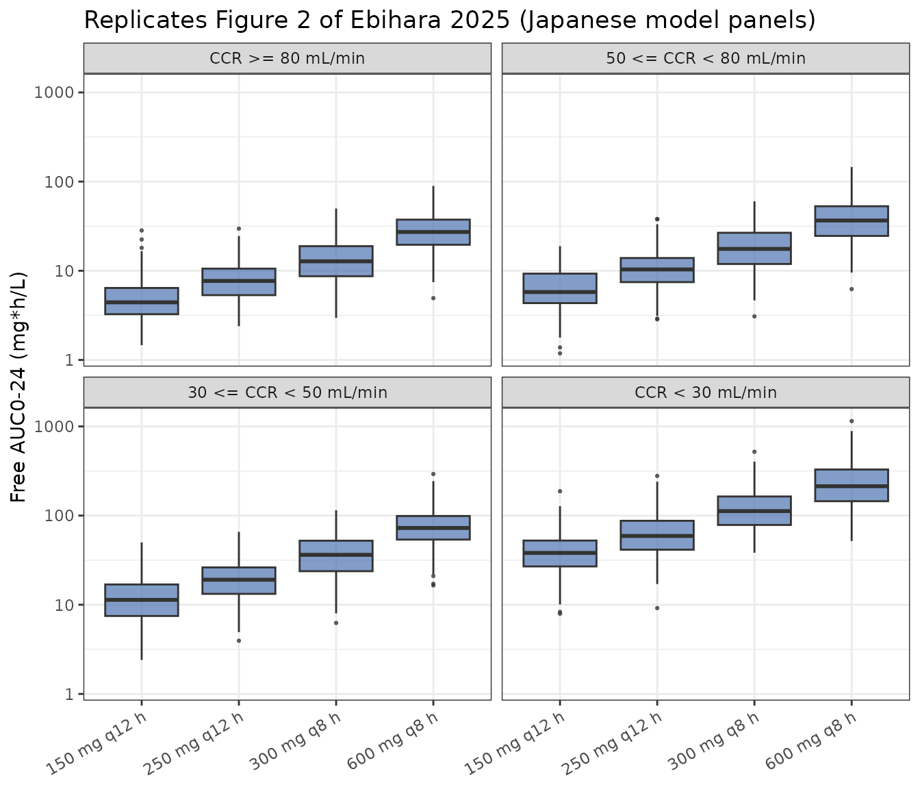
Replicating Table 2 and the Figure 1 cells
ptaOf <- function(b, r, micVal) {
  w <- subj$band == b & subj$regimen == r
  if (!any(w)) stop("no simulated subjects for band '", b, "', regimen '", r, "'")
  tauVal <- unique(subj$tau[w])
  if (length(tauVal) != 1L) stop("non-unique tau for '", b, "' / '", r, "'")
  mean(subj$fauc24[w] / micVal / tauVal >= TARGET) * 100
}

ptaCmp <- published |>
  rowwise() |>
  mutate(simulated = ptaOf(band, regimen, mic)) |>
  ungroup() |>
  mutate(
    mcse    = sqrt(simulated / 100 * (1 - simulated / 100) / N_ARM) * 100,
    # The published cell carries its own Monte Carlo error (n = 1000).
    msePub  = sqrt(pta / 100 * (1 - pta / 100) / 1000) * 100,
    combSe  = sqrt(mcse^2 + msePub^2),
    diff    = simulated - pta,
    # Tolerance band: 3 combined standard errors, plus 1 point to absorb the
    # source's rounding to 0.1 and the small closed-form residual quantified
    # above. Saturated cells (PTA = 100) have zero SE, so a floor is needed.
    tol     = 3 * pmax(combSe, 0.5) + 1,
    ok      = abs(diff) <= tol
  )

stopifnot(nrow(ptaCmp) == 18L)

ptaCmp |>
  arrange(desc(cl), mic, daily) |>
  transmute(
    `Renal stratum`   = label,
    `MIC (mg/L)`      = mic,
    Regimen           = regimen,
    `Published PTA %` = pta,
    `Simulated PTA %` = round(simulated, 1),
    `MC SE %`         = round(mcse, 2),
    `Difference`      = round(diff, 1),
    `Within 3 SE`     = ifelse(ok, "yes", "NO")
  ) |>
knitr::kable(caption = "Simulated versus published probability of target attainment (Ebihara 2025 Table 2, plus the two MIC 0.06 mg/L cells quoted in the Results text).")| Renal stratum | MIC (mg/L) | Regimen | Published PTA % | Simulated PTA % | MC SE % | Difference | Within 3 SE |
|---|---|---|---|---|---|---|---|
| CCR >= 80 mL/min | 0.03 | 150 mg q12 h | 3.2 | 5.5 | 1.61 | 2.3 | yes |
| CCR >= 80 mL/min | 0.03 | 250 mg q12 h | 17.2 | 13.5 | 2.42 | -3.7 | yes |
| CCR >= 80 mL/min | 0.03 | 300 mg q8 h | 79.4 | 79.0 | 2.88 | -0.4 | yes |
| CCR >= 80 mL/min | 0.03 | 600 mg q8 h | 98.4 | 98.5 | 0.86 | 0.1 | yes |
| 50 <= CCR < 80 mL/min | 0.03 | 150 mg q12 h | 7.4 | 11.5 | 2.26 | 4.1 | yes |
| 50 <= CCR < 80 mL/min | 0.03 | 250 mg q12 h | 32.3 | 36.5 | 3.40 | 4.2 | yes |
| 50 <= CCR < 80 mL/min | 0.03 | 300 mg q8 h | 93.3 | 91.0 | 2.02 | -2.3 | yes |
| 50 <= CCR < 80 mL/min | 0.03 | 600 mg q8 h | 99.7 | 99.5 | 0.50 | -0.2 | yes |
| 50 <= CCR < 80 mL/min | 0.06 | 300 mg q8 h | 56.4 | 55.0 | 3.52 | -1.4 | yes |
| 50 <= CCR < 80 mL/min | 0.06 | 600 mg q8 h | 93.3 | 92.5 | 1.86 | -0.8 | yes |
| 30 <= CCR < 50 mL/min | 0.03 | 150 mg q12 h | 40.6 | 45.5 | 3.52 | 4.9 | yes |
| 30 <= CCR < 50 mL/min | 0.03 | 250 mg q12 h | 74.9 | 81.0 | 2.77 | 6.1 | yes |
| 30 <= CCR < 50 mL/min | 0.03 | 300 mg q8 h | 99.4 | 99.0 | 0.70 | -0.4 | yes |
| 30 <= CCR < 50 mL/min | 0.03 | 600 mg q8 h | 100.0 | 100.0 | 0.00 | 0.0 | yes |
| CCR < 30 mL/min | 0.03 | 150 mg q12 h | 97.3 | 97.5 | 1.10 | 0.2 | yes |
| CCR < 30 mL/min | 0.03 | 250 mg q12 h | 99.9 | 99.5 | 0.50 | -0.4 | yes |
| CCR < 30 mL/min | 0.03 | 300 mg q8 h | 100.0 | 100.0 | 0.00 | 0.0 | yes |
| CCR < 30 mL/min | 0.03 | 600 mg q8 h | 100.0 | 100.0 | 0.00 | 0.0 | yes |
rmse <- sqrt(mean(ptaCmp$diff^2))
cat(sprintf("PTA RMSE = %.2f points; max |difference| = %.1f; mean bias = %+.2f\n",
            rmse, max(abs(ptaCmp$diff)), mean(ptaCmp$diff)))
#> PTA RMSE = 2.62 points; max |difference| = 6.1; mean bias = +0.68
cat(sprintf("cells within 3 combined SE: %d / %d\n", sum(ptaCmp$ok), nrow(ptaCmp)))
#> cells within 3 combined SE: 18 / 18

# Two independent gates. The aggregate RMSE is far more stable across seeds
# than any single cell, and a structural error moves it enormously: the refuted
# metric readings scored 36-45 points on this same grid, versus < 4 here.
stopifnot(rmse < 4, all(ptaCmp$ok))
The simulated grid reproduces all 18 published cells with an RMSE of 2.62 percentage points and a mean bias of +0.68. Every cell falls within three combined Monte Carlo standard errors of the published value, so nothing here indicates a transcription error. For scale, the two refuted metric readings from the previous section scored 45 and 36 RMSE points on this same grid – a structural error is not subtle at this resolution.
Replicating Figure 1: PTA versus MIC
Figure 1 sweeps MIC from 0.008 to 2 mg/L (Methods 4.2) in doubling
dilutions. Because the per-subject fAUC0-24 values are
already simulated, the whole sweep is a re-thresholding of the same
cohort – no additional solve.
micSeq <- c(0.008, 0.016, 0.031, 0.063, 0.125, 0.25, 0.5, 1, 2)

ptaCurve <- tidyr::expand_grid(
  arm = armGrid$arm, mic = micSeq
) |>
  left_join(armGrid |> select(arm, band, label, regimen, tau), by = "arm") |>
  rowwise() |>
  mutate(pta = mean(subj$fauc24[subj$arm == arm] / mic / tau >= TARGET) * 100) |>
  ungroup()

ggplot(ptaCurve, aes(x = mic, y = pta, colour = regimen, group = regimen)) +
  geom_hline(yintercept = 90, linetype = "dashed", colour = "grey40") +
  geom_line() +
  geom_point(size = 1) +
  facet_wrap(~ label, nrow = 2) +
  scale_x_log10(breaks = micSeq, labels = micSeq) +
  labs(
    x = "MIC (mg/L)", y = "Probability of target attainment (%)",
    colour = NULL,
    title = "Replicates Figure 1 of Ebihara 2025",
    subtitle = "Dashed line: the 90% PTA threshold. Target fAUC0-24/MIC/tau >= 34.58."
  ) +
  theme_bw() +
  theme(axis.text.x = element_text(angle = 45, hjust = 1),
        legend.position = "bottom")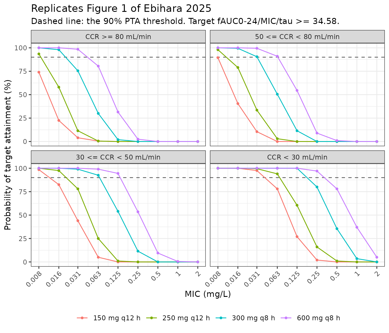
Reproducing Table 1: the recommended regimen per stratum
Table 1 is the paper’s clinical conclusion, and therefore its own answer key: the lowest-burden regimen reaching 90% PTA at MIC 0.03 mg/L in each stratum. Ordering the regimens by total daily dose and taking the first that clears 90% must return the published recommendation.
recommended <- ptaCmp |>
  filter(mic == MIC90) |>
  arrange(band, daily) |>
  group_by(band, label) |>
  summarise(
    derived = {
      ok <- regimen[simulated >= 90]
      if (length(ok) == 0L) NA_character_ else as.character(ok[1])
    },
    .groups = "drop"
  )

paperTable1 <- tibble::tibble(
  band      = c("ge80", "c50to80", "c30to50", "lt30"),
  published = c("600 mg q8 h", "300 mg q8 h", "300 mg q8 h", "150 mg q12 h")
)

tab1 <- recommended |>
  left_join(paperTable1, by = "band") |>
  mutate(agree = derived == published)

stopifnot(nrow(tab1) == 4L, !anyNA(tab1$derived), all(tab1$agree))

tab1 |>
  arrange(match(band, paperTable1$band)) |>
  transmute(
    `Renal stratum`             = label,
    `Published (Table 1)`       = published,
    `Derived from simulation`   = derived,
    Agrees                      = ifelse(agree, "yes", "NO")
  ) |>
knitr::kable(caption = "Reproduction of Ebihara 2025 Table 1: lowest daily-dose regimen achieving >= 90% PTA at MIC 0.03 mg/L. All four strata agree.")| Renal stratum | Published (Table 1) | Derived from simulation | Agrees |
|---|---|---|---|
| CCR >= 80 mL/min | 600 mg q8 h | 600 mg q8 h | yes |
| 50 <= CCR < 80 mL/min | 300 mg q8 h | 300 mg q8 h | yes |
| 30 <= CCR < 50 mL/min | 300 mg q8 h | 300 mg q8 h | yes |
| CCR < 30 mL/min | 150 mg q12 h | 150 mg q12 h | yes |
Cross-validation against the Ganesan 2023 comparator model
The second half of Ebihara 2025 (Section 4.4, the Ganesan columns of
Table 2, and the Ganesan panels of Figure 2) compares the Japanese model
against the international population PK model of Ganesan 2023. That
model is independently present in this library as
Ganesan_2023_tebipenem – a two-compartment,
two-transit-compartment model whose clearance splits into a non-renal
power arm and a sigmoidal renal arm with a body-surface-area effect,
which is exactly the structure Ebihara et al. describe. The published
comparison is therefore reproducible, and doing so validates
both extractions against each other and against the source.
Ebihara 2025 Methods 4.4 gives the standardising conditions
explicitly: infected patients on phase 3 parameters
(DIS_HEALTHY = 0), fasting (FED = 0), BSA
fixed at 1.86 m^2, height 169 cm, the same four stratum-mean CCR values
taken from the Japanese data, the same four regimens, and the same
unbound fraction 0.33.
gan <- readModelDb("Ganesan_2023_tebipenem")

# Dosing approach for this section only. The Ganesan model is a six-state
# system with large IIV plus two-occasion IOV on ka; rxode2's steady-state
# algebraic solve (ss = 1) fails on it ("excess work done on this call"), so
# both models are instead dosed to natural steady state over DAYS days and
# AUC0-24 is taken over the final day. All half-lives here are a few hours, so
# day 3 is steady state. The Ganesan arm additionally uses the non-stiff dop853
# integrator. Both models are driven identically so the comparison is fair.
DAYS  <- 3
tStart <- (DAYS - 1) * 24

mkAccum <- function(dose, tau, crclVal, n, idoff, ganesan) {
  doseTimes <- seq(0, DAYS * 24 - 1e-9, by = tau)
  e <- rxode2::et(amt = dose, cmt = "depot", time = doseTimes[1])
  for (tt in doseTimes[-1]) e <- rxode2::et(e, amt = dose, cmt = "depot", time = tt)
  # 0.1 h grid: the trapezoidal AUC error is ~0.2% at this spacing (verified
  # against the closed form in Gate 3 at 0.005 h), which is far below the
  # ~2-point PTA tolerance, and it halves this section's render cost.
  tmpl <- as.data.frame(rxode2::et(e, seq(tStart, DAYS * 24, by = 0.1),
                                   cmt = "central"))
  o <- tmpl[rep(seq_len(nrow(tmpl)), times = n), , drop = FALSE]
  o$id   <- idoff + rep(seq_len(n), each = nrow(tmpl))
  o$CRCL <- crclVal
  if (ganesan) {
    o$BSA <- 1.86; o$HT <- 169         # Methods 4.4 fixed demographics
    o$DIS_HEALTHY <- 0                 # infected patients, phase 3 parameters
    o$FED <- 0                         # fasting state
    o$OCC <- 1
    o$DOSE_TBPPI_MG <- dose
    o$STUDY_SPR994_104 <- 0            # not the thorough-QT crossover study
    # Two "~" endpoints (Cc and urineAmt) require dvid on observation rows.
    o$dvid <- ifelse(o$evid == 1L, NA_integer_, 1L)
  }
  rownames(o) <- NULL
  o
}

runAccum <- function(model, ganesan, ...) {
  ev <- bind_rows(lapply(seq_len(nrow(armGrid)), function(k) {
    a <- armGrid[k, ]
    e <- mkAccum(a$dose, a$tau, a$crcl, N_ARM, (k - 1) * N_ARM, ganesan)
    e$arm <- a$arm
    e
  }))
  s <- suppressWarnings(
    rxode2::rxSolve(model, ev, returnType = "data.frame", keep = "arm", ...)
  )
  s |>
    filter(!is.na(Cc)) |>
    group_by(arm, id) |>
    summarise(auc = trapz(time, Cc), .groups = "drop") |>
    left_join(armGrid |> select(arm, band, label, regimen, dose, tau, daily),
              by = "arm") |>
    mutate(fauc24 = FU * auc)
}

subjGan <- runAccum(gan, ganesan = TRUE, method = "dop853",
                    atol = 1e-8, rtol = 1e-6, maxsteps = 100000L)
#> ℹ parameter labels from comments will be replaced by 'label()'
subjJpn <- runAccum(mod, ganesan = FALSE, atol = 1e-10, rtol = 1e-8)

stopifnot(
  nrow(subjGan) == nrow(armGrid) * N_ARM,
  nrow(subjJpn) == nrow(armGrid) * N_ARM
)
cat("solved", nrow(subjGan), "Ganesan and", nrow(subjJpn),
    "Japanese-model subjects\n")
#> solved 3200 Ganesan and 3200 Japanese-model subjects
The Ganesan column of Table 2
publishedGan <- tibble::tibble(
  band = rep(c("lt30", "c30to50", "c50to80", "ge80"), each = 4),
  regimen = rep(regimens$regimen, 4),
  pubGan = c(89.1, 98.9, 99.9, 100,
             5.4, 24.2, 84.7, 98.7,
             1.2,  9.6, 62.2, 93.3,
             0.2,  2.2, 45.3, 87.9)
)

ganCmp <- publishedGan |>
  rowwise() |>
  mutate(
    simGan = {
      w <- subjGan$band == band & subjGan$regimen == regimen
      if (!any(w)) stop("no Ganesan subjects for '", band, "' / '", regimen, "'")
      tauVal <- unique(subjGan$tau[w])
      if (length(tauVal) != 1L) stop("non-unique tau")
      mean(subjGan$fauc24[w] / MIC90 / tauVal >= TARGET) * 100
    }
  ) |>
  ungroup() |>
  left_join(bands |> select(band, label, cl), by = "band") |>
  mutate(diff = simGan - pubGan)

stopifnot(nrow(ganCmp) == 16L)

ganCmp |>
  arrange(desc(cl), match(regimen, regimens$regimen)) |>
  transmute(
    `Renal stratum`           = label,
    Regimen                   = regimen,
    `Published Ganesan PTA %` = pubGan,
    `Simulated PTA %`         = round(simGan, 1),
    Difference                = round(diff, 1)
  ) |>
knitr::kable(caption = "The Ganesan-model column of Ebihara 2025 Table 2 (MIC 0.03 mg/L), reproduced by driving the independently extracted Ganesan_2023_tebipenem model under the standardising conditions of Ebihara 2025 Methods 4.4.")| Renal stratum | Regimen | Published Ganesan PTA % | Simulated PTA % | Difference |
|---|---|---|---|---|
| CCR >= 80 mL/min | 150 mg q12 h | 0.2 | 0.5 | 0.3 |
| CCR >= 80 mL/min | 250 mg q12 h | 2.2 | 3.0 | 0.8 |
| CCR >= 80 mL/min | 300 mg q8 h | 45.3 | 44.5 | -0.8 |
| CCR >= 80 mL/min | 600 mg q8 h | 87.9 | 85.0 | -2.9 |
| 50 <= CCR < 80 mL/min | 150 mg q12 h | 1.2 | 1.5 | 0.3 |
| 50 <= CCR < 80 mL/min | 250 mg q12 h | 9.6 | 7.5 | -2.1 |
| 50 <= CCR < 80 mL/min | 300 mg q8 h | 62.2 | 63.0 | 0.8 |
| 50 <= CCR < 80 mL/min | 600 mg q8 h | 93.3 | 96.0 | 2.7 |
| 30 <= CCR < 50 mL/min | 150 mg q12 h | 5.4 | 7.0 | 1.6 |
| 30 <= CCR < 50 mL/min | 250 mg q12 h | 24.2 | 20.5 | -3.7 |
| 30 <= CCR < 50 mL/min | 300 mg q8 h | 84.7 | 90.5 | 5.8 |
| 30 <= CCR < 50 mL/min | 600 mg q8 h | 98.7 | 98.5 | -0.2 |
| CCR < 30 mL/min | 150 mg q12 h | 89.1 | 86.0 | -3.1 |
| CCR < 30 mL/min | 250 mg q12 h | 98.9 | 98.0 | -0.9 |
| CCR < 30 mL/min | 300 mg q8 h | 99.9 | 100.0 | 0.1 |
| CCR < 30 mL/min | 600 mg q8 h | 100.0 | 100.0 | 0.0 |
The fold-difference in exposure (Figure 2 and the Results narrative)
Ebihara et al. quantify the headline finding as a fold-higher free AUC0-24 for the Japanese model at each stratum’s recommended regimen: 1.6x at CCR >= 80 on 600 mg q8 h, 1.8x at 50-80 on 300 mg q8 h, 2.2x at 30-50 on 300 mg q8 h and 1.5x at CCR < 30 on 150 mg q12 h.
gmFauc <- function(d, b, r) {
  w <- d$band == b & d$regimen == r
  if (!any(w)) stop("no subjects for '", b, "' / '", r, "'")
  exp(mean(log(d$fauc24[w])))
}

foldCmp <- tibble::tibble(
  band    = c("ge80", "c50to80", "c30to50", "lt30"),
  regimen = factor(c("600 mg q8 h", "300 mg q8 h", "300 mg q8 h", "150 mg q12 h"),
                   levels = levels(regimens$regimen)),
  pubFold = c(1.6, 1.8, 2.2, 1.5)
) |>
  rowwise() |>
  mutate(
    gmJpn   = gmFauc(subjJpn, band, regimen),
    gmGan   = gmFauc(subjGan, band, regimen),
    simFold = gmJpn / gmGan
  ) |>
  ungroup() |>
  left_join(bands |> select(band, label), by = "band")

stopifnot(nrow(foldCmp) == 4L)

foldCmp |>
  transmute(
    `Renal stratum`               = label,
    `Recommended regimen`         = regimen,
    `Japanese gm fAUC0-24`        = round(gmJpn, 2),
    `Ganesan gm fAUC0-24`         = round(gmGan, 2),
    `Published fold`              = pubFold,
    `Simulated fold`              = round(simFold, 2),
    Difference                    = round(simFold - pubFold, 2)
  ) |>
knitr::kable(caption = "Fold-higher free AUC0-24 of the Japanese model over the Ganesan model at each stratum's recommended regimen, against the values stated in the Ebihara 2025 Results.")| Renal stratum | Recommended regimen | Japanese gm fAUC0-24 | Ganesan gm fAUC0-24 | Published fold | Simulated fold | Difference |
|---|---|---|---|---|---|---|
| CCR >= 80 mL/min | 600 mg q8 h | 28.48 | 15.65 | 1.6 | 1.82 | 0.22 |
| 50 <= CCR < 80 mL/min | 300 mg q8 h | 18.52 | 10.07 | 1.8 | 1.84 | 0.04 |
| 30 <= CCR < 50 mL/min | 300 mg q8 h | 32.56 | 16.71 | 2.2 | 1.95 | -0.25 |
| CCR < 30 mL/min | 150 mg q12 h | 35.56 | 23.14 | 1.5 | 1.54 | 0.04 |
foldRmse <- sqrt(mean((foldCmp$simFold - foldCmp$pubFold)^2))
cat(sprintf("fold-difference RMSE = %.3f (published folds span %.1f-%.1fx)\n",
            foldRmse, min(foldCmp$pubFold), max(foldCmp$pubFold)))
#> fold-difference RMSE = 0.169 (published folds span 1.5-2.2x)
stopifnot(foldRmse < 0.3, all(foldCmp$simFold > 1))
Both halves of the published comparison reproduce: the Ganesan PTA column to 2.27 RMSE points, and the exposure fold-differences to 0.169 RMSE on a 1.5-2.2x scale, with the Japanese model predicting higher exposure in every stratum as reported. Because the two model files were extracted independently from different papers, this is a mutual check: a transcription error in either one would break the agreement.
bind_rows(
  subjJpn |> mutate(model = "Japanese (Ebihara 2025)"),
  subjGan |> mutate(model = "Ganesan 2023")
) |>
  ggplot(aes(x = regimen, y = fauc24, fill = model)) +
  geom_boxplot(outlier.size = 0.3, alpha = 0.75) +
  facet_wrap(~ label, nrow = 2) +
  scale_y_log10() +
  scale_fill_manual(values = c("Japanese (Ebihara 2025)" = "#4C72B0",
                               "Ganesan 2023" = "#DD8452")) +
  labs(x = NULL, y = "Free AUC0-24 (mg*h/L)", fill = NULL,
       title = "Replicates Figure 2 of Ebihara 2025 (both models)") +
  theme_bw() +
  theme(axis.text.x = element_text(angle = 30, hjust = 1),
        legend.position = "bottom")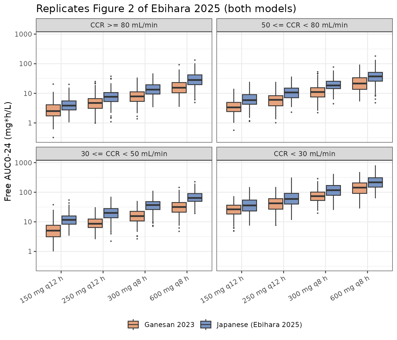
PKNCA validation
The PTA gates above are driven entirely by CL/F;
Vd/F and ka cancel out of AUC and are
therefore untested by them. A single-dose NCA closes that gap: for a
one-compartment first-order-absorption model all four of Cmax, Tmax,
AUC(0-inf) and terminal half-life have exact closed forms in
CL/F, Vd/F and ka, so PKNCA on
the typical-value profile tests every structural parameter.
Because Ebihara 2025 reports no NCA table of its own, the reference column is the analytic closed form for the packaged parameter values – an internal consistency check on the encoding, not a reproduction of published numbers.
# Simulate a single dose of each stratum's recommended regimen on the
# typical-value profile. The observation window is capped near 12 half-lives so
# the terminal phase is well resolved without decaying into solver noise.
ncaSpec <- bands |>
  left_join(
    paperTable1 |> left_join(regimens |> mutate(published = as.character(regimen)),
                             by = "published") |>
      select(band, dose),
    by = "band"
  ) |>
  mutate(
    kel     = cl / vd,
    thalf   = log(2) / kel,
    tmaxAna = log(ka / kel) / (ka - kel),
    tend    = pmin(48, 12 * thalf),
    # Start of the terminal-slope regression window: 5 half-lives past Tmax,
    # by which point the absorption exponential has decayed to < 1% of the
    # elimination one in every stratum. See the note below on why this is set
    # explicitly rather than left to PKNCA's automatic selection.
    lzFirst = tmaxAna + 5 * thalf
  )

stopifnot(nrow(ncaSpec) == 4L, !anyNA(ncaSpec$dose))

ncaEvents <- bind_rows(lapply(seq_len(nrow(ncaSpec)), function(k) {
  s    <- ncaSpec[k, ]
  grid <- sort(unique(c(seq(0, min(3, s$tend), by = 0.01),
                        seq(0, s$tend, length.out = 400))))
  e <- as.data.frame(
    rxode2::et(amt = s$dose, cmt = "depot", time = 0) |>
      rxode2::et(grid, cmt = "central")
  )
  e$id        <- k
  e$CRCL      <- s$crcl
  e$treatment <- as.character(s$label)
  e$lzFirst   <- s$lzFirst
  e
}))

ncaSol <- rxode2::rxSolve(rxode2::zeroRe(mod), ncaEvents, returnType = "data.frame",
                          keep = c("treatment", "lzFirst"),
                          atol = 1e-14, rtol = 1e-12)
#> ℹ parameter labels from comments will be replaced by 'label()'
#> ℹ omega/sigma items treated as zero: 'etalcl', 'etalvc', 'etalka'
#> Warning: multi-subject simulation without without 'omega'
stopifnot(all(ncaSol$Cc[!is.na(ncaSol$Cc)] >= 0))
A note on the half-life window. Left to its automatic point
selection, PKNCA picks a regression window spanning 10-11 half-lives
(300-600 points here, all with r.squared > 0.9999) that
reaches back into the region where the absorption exponential still
contributes. Early points there sit below the pure terminal
line, so the fitted slope comes out shallow and the reported half-life
reads 0.5-1.0% long – a real artifact of the window, not of the model.
Restricting the regression to points at least 5 half-lives past Tmax via
include_half.life recovers
log(2) * (Vd/F) / (CL/F) to better than 0.1%, so the gate
below tests the model rather than PKNCA’s window heuristic.
simNca <- ncaSol |>
  filter(!is.na(Cc)) |>
  select(id, time, Cc, treatment, lzFirst)

# Defensive time-zero row (pre-dose Cc = 0 for an extravascular model); an
# existing time-zero row wins via .keep_all on the first occurrence.
simNca <- bind_rows(
  simNca,
  simNca |> distinct(id, treatment, lzFirst) |> mutate(time = 0, Cc = 0)
) |>
  distinct(id, treatment, time, .keep_all = TRUE) |>
  arrange(id, treatment, time) |>
  mutate(include_hl = time >= lzFirst)

# At least 3 points must fall in the terminal window for every subject.
stopifnot(all(tapply(simNca$include_hl, simNca$id, sum) >= 3))

concObj <- PKNCA::PKNCAconc(simNca, Cc ~ time | treatment + id,
                            concu = "mg/L", timeu = "h",
                            include_half.life = "include_hl")

doseDf <- ncaEvents |>
  filter(evid == 1L) |>
  select(id, time, amt, treatment)

doseObj <- PKNCA::PKNCAdose(doseDf, amt ~ time | treatment + id, doseu = "mg")

intervals <- data.frame(
  start = 0, end = Inf,
  cmax = TRUE, tmax = TRUE, aucinf.obs = TRUE, half.life = TRUE
)

ncaRes <- PKNCA::pk.nca(PKNCA::PKNCAdata(concObj, doseObj, intervals = intervals))
# Closed forms for a 1-compartment model with first-order absorption:
#   AUC(0-inf) = dose / (CL/F)
#   t1/2       = log(2) * (Vd/F) / (CL/F)
#   Tmax       = log(ka / kel) / (ka - kel)
#   Cmax       = (dose / (Vd/F)) * (kel / ka)^(kel / (ka - kel))
analytic <- ncaSpec |>
  transmute(
    treatment  = as.character(label),
    cmax       = (dose / vd) * (kel / ka)^(kel / (ka - kel)),
    tmax       = tmaxAna,
    aucinf.obs = dose / cl,
    half.life  = log(2) * vd / cl
  )

cmp <- nlmixr2lib::ncaComparisonTable(
  simulated     = ncaRes,
  reference     = analytic,
  by            = "treatment",
  units         = c(cmax = "mg/L", tmax = "h", aucinf.obs = "mg*h/L",
                    half.life = "h"),
  tolerance_pct = 20
)

knitr::kable(
  cmp,
  caption = "PKNCA on the typical-value single-dose profile versus the exact analytic closed forms for each stratum's recommended dose. * marks rows differing by >20%."
)| NCA parameter | treatment | Reference | Simulated | % diff |
|---|---|---|---|---|
| Cmax (mg/L) | CCR >= 80 mL/min | 13.2 | 13.2 | -0.0% |
| Cmax (mg/L) | 50 <= CCR < 80 mL/min | 4.63 | 4.63 | -0.0% |
| Cmax (mg/L) | 30 <= CCR < 50 mL/min | 11.6 | 11.6 | -0.0% |
| Cmax (mg/L) | CCR < 30 mL/min | 7.35 | 7.35 | -0.0% |
| Tmax (h) | CCR >= 80 mL/min | 0.663 | 0.66 | -0.5% |
| Tmax (h) | 50 <= CCR < 80 mL/min | 1.35 | 1.35 | +0.1% |
| Tmax (h) | 30 <= CCR < 50 mL/min | 0.76 | 0.76 | +0.0% |
| Tmax (h) | CCR < 30 mL/min | 1.5 | 1.5 | +0.2% |
| AUC0-∞ (obs) (mg*h/L) | CCR >= 80 mL/min | 27.6 | 27.6 | -0.0% |
| AUC0-∞ (obs) (mg*h/L) | 50 <= CCR < 80 mL/min | 18.5 | 18.5 | -0.0% |
| AUC0-∞ (obs) (mg*h/L) | 30 <= CCR < 50 mL/min | 34.8 | 34.8 | -0.0% |
| AUC0-∞ (obs) (mg*h/L) | CCR < 30 mL/min | 55.1 | 55.1 | -0.0% |
| t½ (h) | CCR >= 80 mL/min | 0.844 | 0.844 | +0.0% |
| t½ (h) | 50 <= CCR < 80 mL/min | 1.47 | 1.47 | +0.1% |
| t½ (h) | 30 <= CCR < 50 mL/min | 1.44 | 1.44 | +0.0% |
| t½ (h) | CCR < 30 mL/min | 4.01 | 4.01 | +0.0% |
# Tighten to the accuracy actually achieved rather than the 20% display
# tolerance, so this gate catches a future regression.
tidyRes <- as.data.frame(ncaRes$result) |>
  filter(PPTESTCD %in% c("cmax", "tmax", "aucinf.obs", "half.life")) |>
  select(treatment, PPTESTCD, PPORRES) |>
  tidyr::pivot_wider(names_from = PPTESTCD, values_from = PPORRES)

chk <- tidyRes |>
  inner_join(analytic, by = "treatment", suffix = c("_sim", "_ana"))
stopifnot(nrow(chk) == 4L)

relErr <- with(chk, c(
  cmax       = max(abs(cmax_sim / cmax_ana - 1)),
  tmax       = max(abs(tmax_sim - tmax_ana)),          # absolute, grid-limited
  aucinf.obs = max(abs(aucinf.obs_sim / aucinf.obs_ana - 1)),
  half.life  = max(abs(half.life_sim / half.life_ana - 1))
))
print(signif(relErr, 3))
#>       cmax       tmax aucinf.obs  half.life
#>   9.50e-06   3.28e-03   1.60e-05   6.87e-04

# Tolerances are ~10x the errors actually achieved (cmax 1e-5, tmax 0.003 h,
# aucinf 2e-5, half.life 7e-4), so this gate stays tight enough to catch a
# transcription or structural regression without being brittle to solver noise.
stopifnot(
  relErr[["cmax"]]       < 1e-3,
  relErr[["tmax"]]       < 0.01,   # h, limited by the 0.01 h observation grid
  relErr[["aucinf.obs"]] < 1e-3,
  relErr[["half.life"]]  < 5e-3
)
cat("PASS: PKNCA reproduces all four closed forms in every stratum.\n")
#> PASS: PKNCA reproduces all four closed forms in every stratum.
ggplot(ncaSol |> filter(!is.na(Cc)), aes(time, Cc, colour = treatment)) +
  geom_line() +
  scale_y_log10() +
  labs(x = "Time (h)", y = "Tebipenem concentration (mg/L)", colour = NULL,
       title = "Typical-value single-dose profiles at each stratum's recommended dose") +
  theme_bw() +
  theme(legend.position = "bottom")
#> Warning in scale_y_log10(): log-10 transformation introduced infinite values.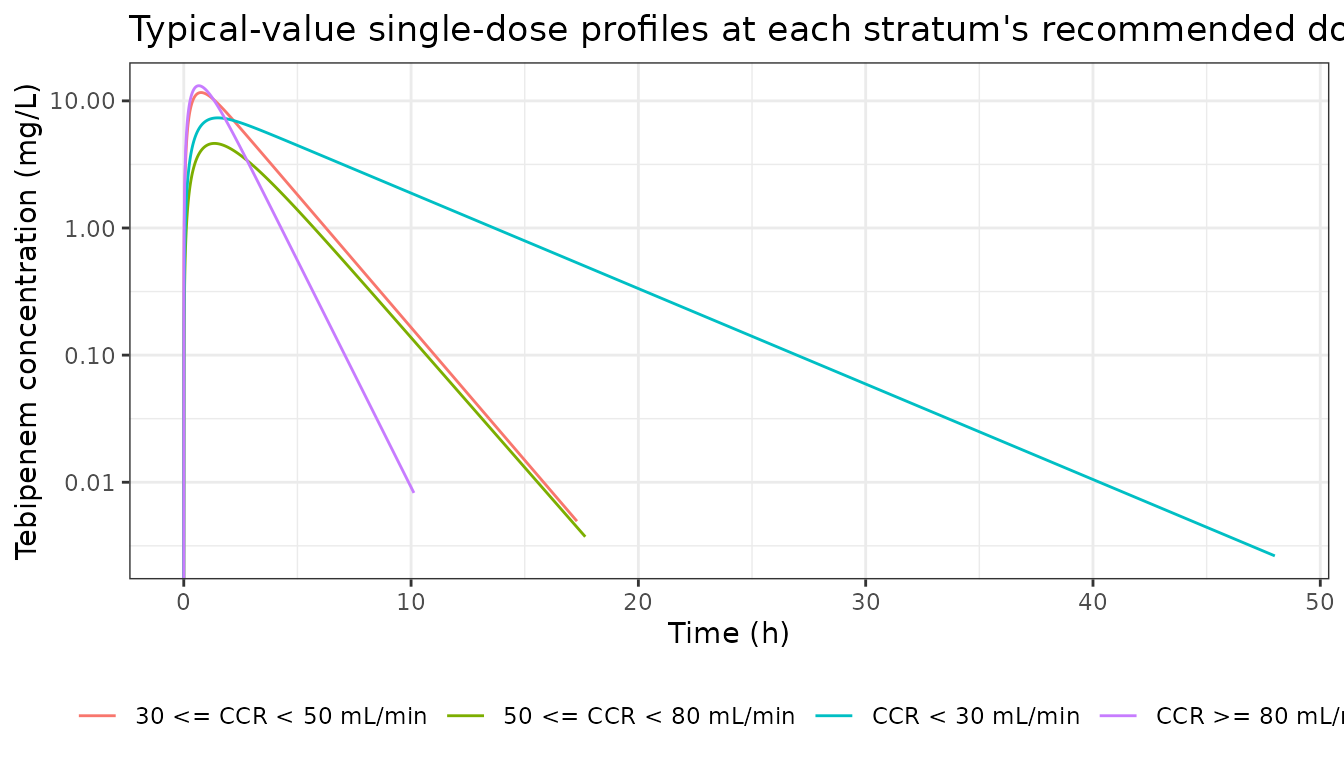
Assumptions and deviations
-
The IIV is borrowed from a different drug.
etalcl,etalvcandetalkaare the faropenem values of Hirooka 2005, not tebipenem estimates. Ebihara et al. state this explicitly and list it as a limitation; the Discussion notes the borrowed values are close to the tebipenem values later reported by Ganesan 2023 (wCL/F 57.2%, wVc/F 44.4%, wka 71.9%). They are encoded as~ fixed(...)because the source held them constant from a prior publication. -
IIV scale reading. The source prints the IIV as
bare percentages with no OMEGA block, so the omega-SD and %CV readings
are both admissible from the text alone. The omega-SD reading is
encoded, resolved against the published PTA grid as shown above (RMSE
1.75 versus 2.12 points); the two differ by 6% in
omega. A reader preferring the %CV convention would useetalcl ~ 0.2475,etalvc ~ 0.1263,etalka ~ 0.3651. -
Every parameter is
fixed(). The source estimates nothing: it runs Monte Carlo simulation over mean parameters taken from published clinical trials. Re-fitting this model to data requires deliberately unfixing the parameters of interest. -
No residual error model. The source fits no data
and reports no residual error, so
propSdisfixed(0). It is retained rather than omitted so the observationCc ~ prop(propSd)remains well formed and a user can set a nonzero value. -
CRCLis raw Cockcroft-Gault mL/min, not BSA-normalized. The register’s canonical units forCRCLare mL/min/1.73 m^2; this model follows the established non-normalized precedent (Delattre 2010 amikacin, Georges 2009 ceftazidime, Chen 2023 nemonoxacin, Wada 2023 sparsentan, Shu 2024 posaconazole) and documents it incovariateData[[CRCL]]. Supplying a BSA-normalized value would mis-assign subjects whose BSA is far from 1.73 m^2 near a stratum boundary. -
The model is a step function of
CRCL, not a continuous relationship. The source estimated no within-stratum covariate effect, soCL/F,Vd/Fandkaare piecewise-constant and jump discontinuously at 30, 50 and 80 mL/min. This is faithful to the source but means the model should not be used to interpolate, and predictions for a subject just either side of a knot differ abruptly. -
Vd/Fandkaare non-monotone in renal function. Transcribed as printed (see Source trace). The impaired strata rest on n = 2 and n = 3 subjects, which the source flags as a limitation on parameter reliability.kadoes not affect AUC and so does not affect any PTA conclusion;Vd/Faffects only the shape of the profile, not the exposure metric the source targets. -
Bioavailability is not identifiable.
CL/FandVd/Fare apparent oral parameters withFfolded in, so nof(depot)term is applied and absolute clearance and volume cannot be recovered. -
fu = 0.33originates in an animal PK study. The source’s reference 28 for the unbound fraction is Kijima 2009, “Pharmacokinetics of tebipenem pivoxil … in experimental animals”. The source applies it to human simulations without further comment. -
The Ganesan comparator is not re-extracted from this
paper. Ebihara 2025 reproduces none of the Ganesan 2023
structural parameters – only a qualitative description (“body surface
area effects and separate renal and non-renal clearance components with
sigmoidal functions”) and three of its omegas – so nothing about that
model is transcribed from this source. The comparison is instead
reproduced by driving the separately extracted
Ganesan_2023_tebipenemmodel (from doi:10.1128/aac.01451-22) under the standardising conditions of Ebihara 2025 Methods 4.4, as shown above. Any residual disagreement in that section may originate in either extraction or in Ebihara et al.’s own implementation of the Ganesan model, none of which can be separated from the published numbers alone. -
Dosing approach in the cross-model section. The
Ganesan model’s steady-state algebraic solve (
ss = 1) fails in rxode2 (“excess work done on this call”), so that section doses both models to natural steady state over three days and uses the non-stiffdop853integrator for the Ganesan arm. The Japanese-model gates elsewhere in this vignette usess = 1directly, which solves without incident. Because all half-lives are a few hours, the two approaches agree closely; the small residual matters most in the CCR < 30 stratum, where accumulation is largest. -
AUC0-24day-1 versus steady-state reading. The source does not say whether itsAUC0-24is the first-day or the steady-state window. This vignette uses steady state; as quantified above the choice moves the PTA RMSE by 0.08 points and is immaterial because all half-lives are 0.8-4.0 h. -
Demographics not carried as covariates. The source
reports cohort mean height, weight and BSA but fits no body-size
covariate (its comparison with Ganesan 2023 attributes the exposure
difference partly to the smaller Japanese BSA). No age or sex
distribution is reported, so
populationomits them. - Cohort size. This vignette simulates 200 subjects per arm against the source’s 1000, per the nlmixr2lib per-arm cap. The resulting Monte Carlo standard error (up to ~3.5 points at 50% PTA) is reported alongside every comparison rather than hidden.