[177Lu]Lu-PSMA-I&T PSA dynamics (Siebinga 2024)
Source:vignettes/articles/Siebinga_2024_lu177psmaIT.Rmd
Siebinga_2024_lu177psmaIT.RmdModel and source
- Citation: Siebinga H, de Wit-van der Veen BJ, de Vries-Huizing DMV, Vogel WV, Hendrikx JJMA, Huitema ADR. Quantification of biochemical PSA dynamics after radioligand therapy with [177Lu]Lu-PSMA-I&T using a population pharmacokinetic/pharmacodynamic model. EJNMMI Phys. 2024;11(1):39. doi:10.1186/s40658-024-00642-2
- Article: https://doi.org/10.1186/s40658-024-00642-2
- PubMed Central: https://www.ncbi.nlm.nih.gov/pmc/articles/PMC11043318/
This is the sequel to Siebinga_2023_lu177psma617 and the
first published PK/PD model that ties radioligand tumor exposure to a
biochemical response measure. The PK layer is a five-compartment
first-order system fitted to 409 quantitative SPECT/CT scans; the PD
layer is a single prostate-specific antigen (PSA) state fitted
sequentially to 566 PSA observations.
The structure (Figure 1 of the paper):
| Paper index | Compartment | nlmixr2lib state | Observed as |
|---|---|---|---|
| 1 | Central | central |
Cc (MBq/L) |
| 2 | Salivary glands (lumped) | salivary_gland |
Asalivary_gland (MBq) |
| 3 | Kidneys (lumped) | kidney |
Akidney (MBq) |
| 4 | Tumor lesions (lumped) | tumor |
Atumor (MBq) |
| 5 | Remaining tissues (lumped) | other |
not observed |
| – | Effect compartment | effect |
not observed |
| – | PSA | PSA |
PSA (ug/L) |
Only the central compartment has a volume (V1 = 10.3 L,
fixed), so it is observed as a concentration and every tissue as a
decay-corrected radioactivity amount. Salivary-gland uptake is the only
saturable process. The PD layer is Equation 12,
d(PSA)/dt = kG * PSA - (Edrug + Edelayed) * PSAwith a direct effect linear in the tumor activity concentration
(Edrug = kD,direct * Ctumor, Equation 9) and a delayed
effect linear in an effect-compartment concentration equilibrating at
ke0.
mod <- readModelDb("Siebinga_2024_lu177psmaIT")
ui <- rxode2::rxode(mod)
#> ℹ parameter labels from comments will be replaced by 'label()'
#> Warning: some etas defaulted to non-mu referenced, possible parsing error: etaiov_kin_tumor_1, etaiov_kin_tumor_2, etaiov_kin_tumor_3, etaiov_kin_tumor_4, etaiov_kin_tumor_5, etaiov_kin_tumor_6, etaiov_kin_tumor_7, etaiov_kin_tumor_8
#> as a work-around try putting the mu-referenced expression on a simple line
ui
#> ── rxode2-based free-form 7-cmt ODE model ──────────────────────────────────────
#> ── Initalization: ──
#> Fixed Effects ($theta):
#> lkel lvc
#> -1.374366 2.332144
#> lkin_salivary_gland lkout_salivary_gland
#> -4.556380 -2.766209
#> lbmax lkin_kidney
#> 4.897840 -3.438899
#> lkout_kidney lkin_tumor
#> -2.772589 -4.638727
#> lkout_tumor lkin_other
#> -4.199705 -1.290984
#> lkout_other e_tum_vol_kin_tumor
#> -3.700952 1.080000
#> e_tum_vol_kin_salivary_gland e_cycle2_kin_tumor
#> 0.091000 0.731000
#> e_cycle3_kin_tumor e_cycle47_kin_tumor
#> 0.498000 0.436000
#> e_wt_vc e_wt_k
#> 1.000000 -0.250000
#> rbase e_tum_vol_rbase
#> 140.000000 57.500000
#> lkgrow lkd_direct
#> -7.804243 -5.698795
#> lke0 lkd_delay
#> -6.660895 -10.325082
#> boxcox_lkgrow propSd
#> -0.822000 0.555000
#> addSd propSd_Asalivary_gland
#> 9.570000 0.397000
#> propSd_Akidney propSd_Atumor
#> 0.319000 0.327000
#> propSd_PSA
#> 0.293000
#>
#> Omega ($omega):
#> etalkel etalkin_kidney etalkin_tumor etalkin_other
#> etalkel 0.1039644 0.0000000 0.0000000 0.0000000
#> etalkin_kidney 0.0000000 0.1057608 0.0000000 0.0000000
#> etalkin_tumor 0.0000000 0.0000000 0.3378684 0.0000000
#> etalkin_other 0.0000000 0.0000000 0.0000000 0.0812859
#> etalbmax 0.0000000 0.0000000 0.0000000 0.0000000
#> etarbase 0.0000000 0.0000000 0.0000000 0.0000000
#> etalkgrow 0.0000000 0.0000000 0.0000000 0.0000000
#> etalkd_direct 0.0000000 0.0000000 0.0000000 0.0000000
#> etalkd_delay 0.0000000 0.0000000 0.0000000 0.0000000
#> etaiov_kin_tumor_1 0.0000000 0.0000000 0.0000000 0.0000000
#> etaiov_kin_tumor_2 0.0000000 0.0000000 0.0000000 0.0000000
#> etaiov_kin_tumor_3 0.0000000 0.0000000 0.0000000 0.0000000
#> etaiov_kin_tumor_4 0.0000000 0.0000000 0.0000000 0.0000000
#> etaiov_kin_tumor_5 0.0000000 0.0000000 0.0000000 0.0000000
#> etaiov_kin_tumor_6 0.0000000 0.0000000 0.0000000 0.0000000
#> etaiov_kin_tumor_7 0.0000000 0.0000000 0.0000000 0.0000000
#> etaiov_kin_tumor_8 0.0000000 0.0000000 0.0000000 0.0000000
#> etalbmax etarbase etalkgrow etalkd_direct etalkd_delay
#> etalkel 0.0000000 0.00000 0.0000000 0.000000 0.0000000
#> etalkin_kidney 0.0000000 0.00000 0.0000000 0.000000 0.0000000
#> etalkin_tumor 0.0000000 0.00000 0.0000000 0.000000 0.0000000
#> etalkin_other 0.0000000 0.00000 0.0000000 0.000000 0.0000000
#> etalbmax 0.3708046 0.00000 0.0000000 0.000000 0.0000000
#> etarbase 0.0000000 1.43606 0.0000000 0.000000 0.0000000
#> etalkgrow 0.0000000 0.00000 0.6022817 0.000000 0.0000000
#> etalkd_direct 0.0000000 0.00000 0.0000000 1.085189 0.0000000
#> etalkd_delay 0.0000000 0.00000 0.0000000 0.000000 0.5685047
#> etaiov_kin_tumor_1 0.0000000 0.00000 0.0000000 0.000000 0.0000000
#> etaiov_kin_tumor_2 0.0000000 0.00000 0.0000000 0.000000 0.0000000
#> etaiov_kin_tumor_3 0.0000000 0.00000 0.0000000 0.000000 0.0000000
#> etaiov_kin_tumor_4 0.0000000 0.00000 0.0000000 0.000000 0.0000000
#> etaiov_kin_tumor_5 0.0000000 0.00000 0.0000000 0.000000 0.0000000
#> etaiov_kin_tumor_6 0.0000000 0.00000 0.0000000 0.000000 0.0000000
#> etaiov_kin_tumor_7 0.0000000 0.00000 0.0000000 0.000000 0.0000000
#> etaiov_kin_tumor_8 0.0000000 0.00000 0.0000000 0.000000 0.0000000
#> etaiov_kin_tumor_1 etaiov_kin_tumor_2 etaiov_kin_tumor_3
#> etalkel 0.0000000 0.0000000 0.0000000
#> etalkin_kidney 0.0000000 0.0000000 0.0000000
#> etalkin_tumor 0.0000000 0.0000000 0.0000000
#> etalkin_other 0.0000000 0.0000000 0.0000000
#> etalbmax 0.0000000 0.0000000 0.0000000
#> etarbase 0.0000000 0.0000000 0.0000000
#> etalkgrow 0.0000000 0.0000000 0.0000000
#> etalkd_direct 0.0000000 0.0000000 0.0000000
#> etalkd_delay 0.0000000 0.0000000 0.0000000
#> etaiov_kin_tumor_1 0.1335549 0.0000000 0.0000000
#> etaiov_kin_tumor_2 0.0000000 0.1335549 0.0000000
#> etaiov_kin_tumor_3 0.0000000 0.0000000 0.1335549
#> etaiov_kin_tumor_4 0.0000000 0.0000000 0.0000000
#> etaiov_kin_tumor_5 0.0000000 0.0000000 0.0000000
#> etaiov_kin_tumor_6 0.0000000 0.0000000 0.0000000
#> etaiov_kin_tumor_7 0.0000000 0.0000000 0.0000000
#> etaiov_kin_tumor_8 0.0000000 0.0000000 0.0000000
#> etaiov_kin_tumor_4 etaiov_kin_tumor_5 etaiov_kin_tumor_6
#> etalkel 0.0000000 0.0000000 0.0000000
#> etalkin_kidney 0.0000000 0.0000000 0.0000000
#> etalkin_tumor 0.0000000 0.0000000 0.0000000
#> etalkin_other 0.0000000 0.0000000 0.0000000
#> etalbmax 0.0000000 0.0000000 0.0000000
#> etarbase 0.0000000 0.0000000 0.0000000
#> etalkgrow 0.0000000 0.0000000 0.0000000
#> etalkd_direct 0.0000000 0.0000000 0.0000000
#> etalkd_delay 0.0000000 0.0000000 0.0000000
#> etaiov_kin_tumor_1 0.0000000 0.0000000 0.0000000
#> etaiov_kin_tumor_2 0.0000000 0.0000000 0.0000000
#> etaiov_kin_tumor_3 0.0000000 0.0000000 0.0000000
#> etaiov_kin_tumor_4 0.1335549 0.0000000 0.0000000
#> etaiov_kin_tumor_5 0.0000000 0.1335549 0.0000000
#> etaiov_kin_tumor_6 0.0000000 0.0000000 0.1335549
#> etaiov_kin_tumor_7 0.0000000 0.0000000 0.0000000
#> etaiov_kin_tumor_8 0.0000000 0.0000000 0.0000000
#> etaiov_kin_tumor_7 etaiov_kin_tumor_8
#> etalkel 0.0000000 0.0000000
#> etalkin_kidney 0.0000000 0.0000000
#> etalkin_tumor 0.0000000 0.0000000
#> etalkin_other 0.0000000 0.0000000
#> etalbmax 0.0000000 0.0000000
#> etarbase 0.0000000 0.0000000
#> etalkgrow 0.0000000 0.0000000
#> etalkd_direct 0.0000000 0.0000000
#> etalkd_delay 0.0000000 0.0000000
#> etaiov_kin_tumor_1 0.0000000 0.0000000
#> etaiov_kin_tumor_2 0.0000000 0.0000000
#> etaiov_kin_tumor_3 0.0000000 0.0000000
#> etaiov_kin_tumor_4 0.0000000 0.0000000
#> etaiov_kin_tumor_5 0.0000000 0.0000000
#> etaiov_kin_tumor_6 0.0000000 0.0000000
#> etaiov_kin_tumor_7 0.1335549 0.0000000
#> etaiov_kin_tumor_8 0.0000000 0.1335549
#> attr(,"lotriLabels")
#> [1] "Table 2 IIV k10 = 33.1% CV -> log(0.331^2 + 1)"
#> [2] "Table 2 IIV k13 = 33.4% CV -> log(0.334^2 + 1)"
#> [3] "Table 2 IIV k14 = 63.4% CV -> log(0.634^2 + 1)"
#> [4] "Table 2 IIV k15 = 29.1% CV -> log(0.291^2 + 1)"
#> [5] "Table 2 IIV Bmax compartment 2 = 67.0% CV -> log(0.670^2 + 1)"
#> [6] "Table 3 IIV baseline PSA = 179% CV -> log(1.79^2 + 1)"
#> [7] "Table 3 IIV kG = 90.9% CV -> log(0.909^2 + 1); this eta is Box-Cox transformed in model()"
#> [8] "Table 3 IIV kD,direct = 140% CV -> log(1.40^2 + 1)"
#> [9] "Table 3 IIV kD,delay = 87.5% CV -> log(0.875^2 + 1)"
#> [10] NA
#> [11] NA
#> [12] NA
#> [13] NA
#> [14] NA
#> [15] NA
#> [16] NA
#> [17] NA
#> attr(,"lotriFix")
#> etalkel etalkin_kidney etalkin_tumor etalkin_other etalbmax
#> etalkel FALSE FALSE FALSE FALSE FALSE
#> etalkin_kidney FALSE FALSE FALSE FALSE FALSE
#> etalkin_tumor FALSE FALSE FALSE FALSE FALSE
#> etalkin_other FALSE FALSE FALSE FALSE FALSE
#> etalbmax FALSE FALSE FALSE FALSE FALSE
#> etarbase FALSE FALSE FALSE FALSE FALSE
#> etalkgrow FALSE FALSE FALSE FALSE FALSE
#> etalkd_direct FALSE FALSE FALSE FALSE FALSE
#> etalkd_delay FALSE FALSE FALSE FALSE FALSE
#> etaiov_kin_tumor_1 FALSE FALSE FALSE FALSE FALSE
#> etaiov_kin_tumor_2 FALSE FALSE FALSE FALSE FALSE
#> etaiov_kin_tumor_3 FALSE FALSE FALSE FALSE FALSE
#> etaiov_kin_tumor_4 FALSE FALSE FALSE FALSE FALSE
#> etaiov_kin_tumor_5 FALSE FALSE FALSE FALSE FALSE
#> etaiov_kin_tumor_6 FALSE FALSE FALSE FALSE FALSE
#> etaiov_kin_tumor_7 FALSE FALSE FALSE FALSE FALSE
#> etaiov_kin_tumor_8 FALSE FALSE FALSE FALSE FALSE
#> etarbase etalkgrow etalkd_direct etalkd_delay
#> etalkel FALSE FALSE FALSE FALSE
#> etalkin_kidney FALSE FALSE FALSE FALSE
#> etalkin_tumor FALSE FALSE FALSE FALSE
#> etalkin_other FALSE FALSE FALSE FALSE
#> etalbmax FALSE FALSE FALSE FALSE
#> etarbase FALSE FALSE FALSE FALSE
#> etalkgrow FALSE FALSE FALSE FALSE
#> etalkd_direct FALSE FALSE FALSE FALSE
#> etalkd_delay FALSE FALSE FALSE FALSE
#> etaiov_kin_tumor_1 FALSE FALSE FALSE FALSE
#> etaiov_kin_tumor_2 FALSE FALSE FALSE FALSE
#> etaiov_kin_tumor_3 FALSE FALSE FALSE FALSE
#> etaiov_kin_tumor_4 FALSE FALSE FALSE FALSE
#> etaiov_kin_tumor_5 FALSE FALSE FALSE FALSE
#> etaiov_kin_tumor_6 FALSE FALSE FALSE FALSE
#> etaiov_kin_tumor_7 FALSE FALSE FALSE FALSE
#> etaiov_kin_tumor_8 FALSE FALSE FALSE FALSE
#> etaiov_kin_tumor_1 etaiov_kin_tumor_2 etaiov_kin_tumor_3
#> etalkel FALSE FALSE FALSE
#> etalkin_kidney FALSE FALSE FALSE
#> etalkin_tumor FALSE FALSE FALSE
#> etalkin_other FALSE FALSE FALSE
#> etalbmax FALSE FALSE FALSE
#> etarbase FALSE FALSE FALSE
#> etalkgrow FALSE FALSE FALSE
#> etalkd_direct FALSE FALSE FALSE
#> etalkd_delay FALSE FALSE FALSE
#> etaiov_kin_tumor_1 FALSE FALSE FALSE
#> etaiov_kin_tumor_2 FALSE TRUE FALSE
#> etaiov_kin_tumor_3 FALSE FALSE TRUE
#> etaiov_kin_tumor_4 FALSE FALSE FALSE
#> etaiov_kin_tumor_5 FALSE FALSE FALSE
#> etaiov_kin_tumor_6 FALSE FALSE FALSE
#> etaiov_kin_tumor_7 FALSE FALSE FALSE
#> etaiov_kin_tumor_8 FALSE FALSE FALSE
#> etaiov_kin_tumor_4 etaiov_kin_tumor_5 etaiov_kin_tumor_6
#> etalkel FALSE FALSE FALSE
#> etalkin_kidney FALSE FALSE FALSE
#> etalkin_tumor FALSE FALSE FALSE
#> etalkin_other FALSE FALSE FALSE
#> etalbmax FALSE FALSE FALSE
#> etarbase FALSE FALSE FALSE
#> etalkgrow FALSE FALSE FALSE
#> etalkd_direct FALSE FALSE FALSE
#> etalkd_delay FALSE FALSE FALSE
#> etaiov_kin_tumor_1 FALSE FALSE FALSE
#> etaiov_kin_tumor_2 FALSE FALSE FALSE
#> etaiov_kin_tumor_3 FALSE FALSE FALSE
#> etaiov_kin_tumor_4 TRUE FALSE FALSE
#> etaiov_kin_tumor_5 FALSE TRUE FALSE
#> etaiov_kin_tumor_6 FALSE FALSE TRUE
#> etaiov_kin_tumor_7 FALSE FALSE FALSE
#> etaiov_kin_tumor_8 FALSE FALSE FALSE
#> etaiov_kin_tumor_7 etaiov_kin_tumor_8
#> etalkel FALSE FALSE
#> etalkin_kidney FALSE FALSE
#> etalkin_tumor FALSE FALSE
#> etalkin_other FALSE FALSE
#> etalbmax FALSE FALSE
#> etarbase FALSE FALSE
#> etalkgrow FALSE FALSE
#> etalkd_direct FALSE FALSE
#> etalkd_delay FALSE FALSE
#> etaiov_kin_tumor_1 FALSE FALSE
#> etaiov_kin_tumor_2 FALSE FALSE
#> etaiov_kin_tumor_3 FALSE FALSE
#> etaiov_kin_tumor_4 FALSE FALSE
#> etaiov_kin_tumor_5 FALSE FALSE
#> etaiov_kin_tumor_6 FALSE FALSE
#> etaiov_kin_tumor_7 TRUE FALSE
#> etaiov_kin_tumor_8 FALSE TRUE
#>
#> States ($state or $stateDf):
#> Compartment Number Compartment Name
#> 1 1 central
#> 2 2 salivary_gland
#> 3 3 kidney
#> 4 4 tumor
#> 5 5 other
#> 6 6 effect
#> 7 7 PSA
#> ── Multiple Endpoint Model ($multipleEndpoint): ──
#> variable cmt
#> 1 Cc ~ … cmt='Cc' or cmt=8
#> 2 Asalivary_gland ~ … cmt='Asalivary_gland' or cmt=9
#> 3 Akidney ~ … cmt='Akidney' or cmt=10
#> 4 Atumor ~ … cmt='Atumor' or cmt=11
#> 5 PSA ~ … cmt='PSA' or cmt=7
#> dvid*
#> 1 dvid='Cc' or dvid=1
#> 2 dvid='Asalivary_gland' or dvid=2
#> 3 dvid='Akidney' or dvid=3
#> 4 dvid='Atumor' or dvid=4
#> 5 dvid='PSA' or dvid=5
#> * If dvids are outside this range, all dvids are re-numered sequentially, ie 1,7, 10 becomes 1,2,3 etc
#>
#> ── μ-referencing ($muRefTable): ──
#> theta eta level
#> 1 lkel etalkel id
#> 2 lbmax etalbmax id
#> 3 lkin_kidney etalkin_kidney id
#> 4 lkin_tumor etalkin_tumor id
#> 5 lkin_other etalkin_other id
#> 6 lkd_direct etalkd_direct id
#> 7 lkd_delay etalkd_delay id
#>
#> ── Model (Normalized Syntax): ──
#> function() {
#> compartmentData <- list(central = list(analyte = "[177Lu]Lu-PSMA-I&T radioactivity",
#> units = "MBq", specimen = "whole blood", verified = TRUE),
#> salivary_gland = list(analyte = "[177Lu]Lu-PSMA-I&T radioactivity",
#> units = "MBq", specimen = "tissue", verified = TRUE),
#> kidney = list(analyte = "[177Lu]Lu-PSMA-I&T radioactivity",
#> units = "MBq", specimen = "tissue", verified = TRUE),
#> tumor = list(analyte = "[177Lu]Lu-PSMA-I&T radioactivity",
#> units = "MBq", specimen = "tumor", verified = TRUE),
#> other = list(analyte = "[177Lu]Lu-PSMA-I&T radioactivity",
#> units = "MBq", specimen = "tissue", verified = FALSE),
#> effect = list(analyte = "[177Lu]Lu-PSMA-I&T effect-compartment activity concentration",
#> units = "MBq/L", specimen = "not applicable", verified = FALSE),
#> PSA = list(analyte = "prostate-specific antigen", units = "ug/L",
#> specimen = "serum", verified = TRUE))
#> covariateData <- list(WT = list(description = "Total body weight at baseline (Table 1 median 79 kg, range 61-116).",
#> units = "kg", type = "continuous", reference_category = NULL,
#> notes = "Allometric scaling was added to all PK parameters (Results, 'Population pharmacokinetic model'; dOFV -11.3). Methods state that body weight was scaled 'in relation to the median body weight, where exponents for volume of distribution (V) and rate constants (k) were set to 1 and -0.25 respectively', so both exponents are fixed a priori rather than estimated and the reference is the Table 1 median of 79 kg. Bmax is neither a volume nor a rate constant and the paper names only V and k, so Bmax is left unscaled. Baseline value, held constant per subject.",
#> source_name = "Weight"), TUM_VOL = list(description = "Tumor volume of the segmented (target) lesions, determined on pre-treatment diagnostic PSMA-PET/CT with a 45% SULmax threshold. Reported in L in Table 1 (median 0.0443 L, range 0.000122-0.546); carried here in the canonical mm^3 (1 L = 1e6 mm^3), so the reference is 44300 mm^3.",
#> units = "mm^3", type = "continuous", reference_category = NULL,
#> notes = "Enters three places. (1) Tumor uptake rate as a power function (Table 2 'Tumor volume on k14' = 1.08); the paper's own check is that a two-fold volume gives a 2.11-fold uptake rate, and 2^1.08 = 2.114. (2) Salivary-gland uptake rate as a power function (Table 2 'Tumor volume on k12' = 0.0910). (3) Baseline PSA as a linear function (Table 3, 57.5 ug/L). The same volume also converts the tumor radioactivity amount to the concentration that drives the PD layer. Only target-lesion volume was available, not total tumor volume (Methods, 'Pharmacokinetic model development'). Baseline value, held constant per subject.",
#> source_name = "Tumor volume of segmented tumors"), CYCLE = list(description = "Treatment-cycle number (1 = first ~7.4 GBq administration). Patients received up to eight cycles (Table 1).",
#> units = "(count)", type = "count", reference_category = NULL,
#> notes = "Carries two distinct effects on the tumor uptake rate constant and is decomposed inside model() into binary indicators rather than entering as an integer. (1) The structural cycle effect of Equation 8: uptake in each cycle is a fraction of the cycle-1 uptake, with cycles 4 and later lumped into a single level because few patients received more than four cycles (Table 2: 0.731, 0.498, 0.436 for cycles 2, 3 and 4-7). (2) The occasion index for interoccasion variability, which the paper added only to the tumor uptake rate (Table 2 IOV k14 = 37.8% CV). Occasions 1-8 are provided to cover the observed range of cycles.",
#> source_name = "Number of cycles received"))
#> covariatesDataExcluded <- list(CRCL = list(description = "Glomerular filtration rate estimated with the Cockcroft-Gault equation (Table 1 median 80.9 mL/min, range 25.9-181).",
#> units = "mL/min", type = "continuous", notes = "Tested as a linear covariate on the renal excretion rate constant k10, which the paper considered pharmacologically the most suitable form because glomerular filtration is the only elimination route. It was not retained: 'Serum creatinine clearance was not identified as a covariate on k10, since the OFV and model fit did not improve (dOFV -0.207)' (Results). No coefficient is reported, so the effect cannot be encoded. Note that the predecessor [177Lu]Lu-PSMA-617 model (Siebinga_2023_lu177psma617.R) did scale k10 by CRCL a priori.",
#> source_name = "GFR (calculated using Cockcroft Gault)"),
#> AGE = list(description = "Age at baseline (Table 1 median 73 years, range 48-91).",
#> units = "years", type = "continuous", notes = "Tested as a power and a linear covariate on baseline PSA on the hypothesis that age tracks disease severity; not retained ('Age did not explain IIV on the baseline PSA (dOFV -1.01)', Results). No coefficient is reported.",
#> source_name = "Age"), HCT = list(description = "Hematocrit at baseline (Table 1 median 0.35, range 0.22-0.44).",
#> units = "(fraction)", type = "continuous", notes = "Reported among the baseline characteristics in Table 1 but never tested as a covariate and not part of any model.",
#> source_name = "Hematocrit"))
#> description <- "Five-compartment population PK model with a sequentially fitted PSA pharmacodynamic layer for the PSMA-targeted radioligand [177Lu]Lu-PSMA-I&T in men with metastatic castration-resistant prostate cancer treated with ~7.4 GBq per cycle. PK states are central (1), salivary glands (2), kidneys (3), tumor lesions (4) and a lumped remaining-tissue compartment (5); the tissue states carry radioactivity amounts (MBq) and the central state is observed as a concentration (MBq/L) through a fixed volume V1 = 10.3 L. Renal excretion leaves the central compartment (k10 = 0.253 1/h, i.e. 2.61 L/h). Salivary-gland uptake is saturable (Bmax 134 MBq); all other exchange is first order. Tumor uptake carries a power effect of segmented tumor volume (exponent 1.08), a structural decline over treatment cycles (73%, 50% and 44% of the cycle-1 rate in cycles 2, 3 and 4-7), interindividual variability (63.4% CV) and interoccasion variability across cycles (37.8% CV), and salivary-gland uptake carries a weak tumor-volume power effect. All PK parameters are allometrically scaled to the 79 kg median body weight. The PD layer is a single PSA state growing exponentially (kG 0.000408 1/h) and eliminated by a direct effect linear in the physical tumor activity concentration plus a delayed effect linear in an effect-compartment concentration (ke0 0.00128 1/h). Baseline PSA is fixed at 140 ug/L with a linear tumor-volume effect. Every state carries a decay-corrected radioactivity amount, matching the source SPECT/CT data and the predecessor [177Lu]Lu-PSMA-617 model."
#> population <- list(species = "human", n_subjects = 76, n_studies = 1,
#> age_range = "48-91 years", age_median = "73 years", weight_range = "61-116 kg",
#> weight_median = "79 kg", sex_female_pct = 0, disease_state = "Metastatic castration-resistant prostate cancer with PSMA-positive lesions on pre-treatment diagnostic [68Ga]Ga-PSMA PET/CT and no PSMA-negative lesions on contrast-enhanced CT (VISION criteria). Baseline PSA median 260 ug/L (0.12-4896); segmented target-tumor volume median 0.0443 L (0.000122-0.546); hematocrit median 0.35.",
#> renal_function = "Cockcroft-Gault GFR median 80.9 mL/min (range 25.9-181)",
#> dose_range = "Intravenous [177Lu]Lu-PSMA-I&T, median injected activity 7378 MBq (5605-7763) per cycle, up to eight cycles. Two schedules were used: four cycles six weeks apart ('4 x 6', n = 10) and two cycles two weeks apart repeated after twelve weeks ('2 x 2 - repeated after twelve weeks', n = 66).",
#> regions = "Netherlands (Netherlands Cancer Institute / Antoni van Leeuwenhoek; IRBd21288)",
#> notes = "Retrospective cohort treated September 2019 to January 2023. The PK model was built on 409 quantitative SPECT/CT scans from 76 patients (3 of 79 screened patients had only lesions < 20 mm and were excluded); scans were acquired at 4.6 +/- 0.95 h, 23.8 +/- 4.5 h and 6.8 +/- 0.46 days post injection. Kidney, salivary-gland and tumor readings were lumped into one state each; whole-body data were not available. All radioactivity data were corrected for decay back to the time of injection, and SPECT-derived blood concentrations were recalibrated with the [177Lu]Lu-PSMA-617 regression (intercept 6.27 MBq/L, slope 0.828) taken from the predecessor model. The PD layer was fitted sequentially to 566 PSA observations.")
#> reference <- "Siebinga H, de Wit-van der Veen BJ, de Vries-Huizing DMV, Vogel WV, Hendrikx JJMA, Huitema ADR. Quantification of biochemical PSA dynamics after radioligand therapy with [177Lu]Lu-PSMA-I&T using a population pharmacokinetic/pharmacodynamic model. EJNMMI Phys. 2024;11(1):39. doi:10.1186/s40658-024-00642-2"
#> units <- list(time = "h", dosing = "MBq", concentration = "MBq/L")
#> vignette <- "Siebinga_2024_lu177psmaIT"
#> ini({
#> lkel <- -1.37436579025462
#> label("Renal excretion rate constant from central, k10 (1/h)")
#> lvc <- fix(2.33214389523559)
#> label("Central volume of distribution, V1 (L)")
#> lkin_salivary_gland <- -4.55638002181866
#> label("Central-to-salivary-gland uptake rate constant, k12 (1/h)")
#> lkout_salivary_gland <- -2.76620911527574
#> label("Salivary-gland-to-central rate constant, k21 (1/h)")
#> lbmax <- 4.89783979995091
#> label("Maximum salivary-gland binding capacity, Bmax (MBq)")
#> lkin_kidney <- -3.43889924884617
#> label("Central-to-kidney uptake rate constant, k13 (1/h)")
#> lkout_kidney <- -2.77258872223978
#> label("Kidney-to-central rate constant, k31 (1/h)")
#> lkin_tumor <- -4.63872696951693
#> label("Central-to-tumor uptake rate constant, k14 (1/h)")
#> lkout_tumor <- -4.19970507787993
#> label("Tumor-to-central rate constant, k41 (1/h)")
#> lkin_other <- -1.29098418131557
#> label("Central-to-remaining-tissue rate constant, k15 (1/h)")
#> lkout_other <- -3.70095203534821
#> label("Remaining-tissue-to-central rate constant, k51 (1/h)")
#> e_tum_vol_kin_tumor <- 1.08
#> label("Power exponent of segmented tumor volume on kin_tumor (unitless)")
#> e_tum_vol_kin_salivary_gland <- 0.091
#> label("Power exponent of segmented tumor volume on kin_salivary_gland (unitless)")
#> e_cycle2_kin_tumor <- 0.731
#> label("Fraction of cycle-1 tumor uptake rate retained in cycle 2 (unitless)")
#> e_cycle3_kin_tumor <- 0.498
#> label("Fraction of cycle-1 tumor uptake rate retained in cycle 3 (unitless)")
#> e_cycle47_kin_tumor <- 0.436
#> label("Fraction of cycle-1 tumor uptake rate retained in cycles 4-7 (unitless)")
#> e_wt_vc <- fix(1)
#> label("Allometric exponent of body weight on the central volume (unitless)")
#> e_wt_k <- fix(-0.25)
#> label("Allometric exponent of body weight on every rate constant (unitless)")
#> rbase <- fix(140)
#> label("Baseline PSA concentration (ug/L)")
#> e_tum_vol_rbase <- 57.5
#> label("Linear effect of segmented tumor volume on baseline PSA (ug/L)")
#> lkgrow <- -7.80424338356011
#> label("First-order exponential PSA growth rate, kG (1/h)")
#> lkd_direct <- -5.69879493314516
#> label("Direct drug-induced PSA elimination coefficient, kD,direct (L/day/GBq)")
#> lke0 <- -6.66089520105061
#> label("Effect-compartment equilibration rate constant, ke0 (1/h)")
#> lkd_delay <- -10.3250820425742
#> label("Delayed drug-induced PSA elimination coefficient, kD,delay (L/day/MBq)")
#> boxcox_lkgrow <- -0.822
#> label("Box-Cox shape parameter for the interindividual distribution of kG (unitless)")
#> propSd <- c(0, 0.555)
#> label("Proportional residual error, central concentration (fraction)")
#> addSd <- c(0, 9.57)
#> label("Additive residual error, central concentration (MBq/L)")
#> propSd_Asalivary_gland <- c(0, 0.397)
#> label("Proportional residual error, salivary-gland activity (fraction)")
#> propSd_Akidney <- c(0, 0.319)
#> label("Proportional residual error, kidney activity (fraction)")
#> propSd_Atumor <- c(0, 0.327)
#> label("Proportional residual error, tumor activity (fraction)")
#> propSd_PSA <- c(0, 0.293)
#> label("Proportional residual error, PSA (fraction)")
#> etalkel ~ 0.1039644
#> label("Table 2 IIV k10 = 33.1% CV -> log(0.331^2 + 1)")
#> etalkin_kidney ~ 0.1057608
#> label("Table 2 IIV k13 = 33.4% CV -> log(0.334^2 + 1)")
#> etalkin_tumor ~ 0.3378684
#> label("Table 2 IIV k14 = 63.4% CV -> log(0.634^2 + 1)")
#> etalkin_other ~ 0.0812859
#> label("Table 2 IIV k15 = 29.1% CV -> log(0.291^2 + 1)")
#> etalbmax ~ 0.3708046
#> label("Table 2 IIV Bmax compartment 2 = 67.0% CV -> log(0.670^2 + 1)")
#> etarbase ~ 1.4360602
#> label("Table 3 IIV baseline PSA = 179% CV -> log(1.79^2 + 1)")
#> etalkgrow ~ 0.6022817
#> label("Table 3 IIV kG = 90.9% CV -> log(0.909^2 + 1); this eta is Box-Cox transformed in model()")
#> etalkd_direct ~ 1.0851893
#> label("Table 3 IIV kD,direct = 140% CV -> log(1.40^2 + 1)")
#> etalkd_delay ~ 0.5685047
#> label("Table 3 IIV kD,delay = 87.5% CV -> log(0.875^2 + 1)")
#> etaiov_kin_tumor_1 ~ 0.1335549
#> etaiov_kin_tumor_2 ~ fix(0.1335549)
#> etaiov_kin_tumor_3 ~ fix(0.1335549)
#> etaiov_kin_tumor_4 ~ fix(0.1335549)
#> etaiov_kin_tumor_5 ~ fix(0.1335549)
#> etaiov_kin_tumor_6 ~ fix(0.1335549)
#> etaiov_kin_tumor_7 ~ fix(0.1335549)
#> etaiov_kin_tumor_8 ~ fix(0.1335549)
#> })
#> model({
#> aloV <- e_wt_vc
#> aloK <- e_wt_k
#> rbasePop <- rbase
#> eTumVolRbase <- e_tum_vol_rbase
#> bcLambda <- boxcox_lkgrow
#> cyc2 <- (CYCLE == 2)
#> cyc3 <- (CYCLE == 3)
#> cyc47 <- (CYCLE >= 4)
#> fcyc2 <- e_cycle2_kin_tumor
#> fcyc3 <- e_cycle3_kin_tumor
#> fcyc47 <- e_cycle47_kin_tumor
#> cycleFactor <- fcyc2^cyc2 * fcyc3^cyc3 * fcyc47^cyc47
#> iov_kin_tumor <- (CYCLE == 1) * etaiov_kin_tumor_1 +
#> (CYCLE == 2) * etaiov_kin_tumor_2 + (CYCLE == 3) *
#> etaiov_kin_tumor_3 + (CYCLE == 4) * etaiov_kin_tumor_4 +
#> (CYCLE == 5) * etaiov_kin_tumor_5 + (CYCLE == 6) *
#> etaiov_kin_tumor_6 + (CYCLE == 7) * etaiov_kin_tumor_7 +
#> (CYCLE >= 8) * etaiov_kin_tumor_8
#> alloV <- (WT/79)^aloV
#> alloK <- (WT/79)^aloK
#> kel <- exp(lkel + etalkel) * alloK
#> vc <- exp(lvc) * alloV
#> kin_salivary_gland <- exp(lkin_salivary_gland) * alloK *
#> (TUM_VOL/44300)^e_tum_vol_kin_salivary_gland
#> kout_salivary_gland <- exp(lkout_salivary_gland) * alloK
#> bmax <- exp(lbmax + etalbmax)
#> kin_kidney <- exp(lkin_kidney + etalkin_kidney) * alloK
#> kout_kidney <- exp(lkout_kidney) * alloK
#> kin_tumor <- exp(lkin_tumor + etalkin_tumor + iov_kin_tumor) *
#> alloK * (TUM_VOL/44300)^e_tum_vol_kin_tumor * cycleFactor
#> kout_tumor <- exp(lkout_tumor) * alloK
#> kin_other <- exp(lkin_other + etalkin_other) * alloK
#> kout_other <- exp(lkout_other) * alloK
#> basePop <- rbasePop + eTumVolRbase * (TUM_VOL/44300)
#> psa0 <- basePop * exp(etarbase)
#> phi_lkgrow <- (exp(etalkgrow)^bcLambda - 1)/bcLambda
#> kgrow <- exp(lkgrow + phi_lkgrow)
#> ke0 <- exp(lke0)
#> kd_direct <- exp(lkd_direct + etalkd_direct)
#> kd_delay <- exp(lkd_delay + etalkd_delay)
#> fluxSalivaryGland <- kin_salivary_gland * central * (1 -
#> salivary_gland/bmax)
#> d/dt(central) <- -kel * central - fluxSalivaryGland +
#> kout_salivary_gland * salivary_gland - kin_kidney *
#> central + kout_kidney * kidney - kin_tumor * central +
#> kout_tumor * tumor - kin_other * central + kout_other *
#> other
#> d/dt(salivary_gland) <- fluxSalivaryGland - kout_salivary_gland *
#> salivary_gland
#> d/dt(kidney) <- kin_kidney * central - kout_kidney *
#> kidney
#> d/dt(tumor) <- kin_tumor * central - kout_tumor * tumor
#> d/dt(other) <- kin_other * central - kout_other * other
#> vtumor <- TUM_VOL/1e+06
#> Ctumor <- tumor/vtumor
#> d/dt(effect) <- ke0 * (Ctumor - effect)
#> edrug <- kd_direct * Ctumor/1000/24
#> edelayed <- kd_delay * effect/24
#> d/dt(PSA) <- kgrow * PSA - (edrug + edelayed) * PSA
#> PSA(0) <- psa0
#> Cc <- central/vc
#> Asalivary_gland <- salivary_gland
#> Akidney <- kidney
#> Atumor <- tumor
#> Cc ~ add(addSd) + prop(propSd)
#> Asalivary_gland ~ prop(propSd_Asalivary_gland)
#> Akidney ~ prop(propSd_Akidney)
#> Atumor ~ prop(propSd_Atumor)
#> PSA ~ prop(propSd_PSA)
#> })
#> }Population
Seventy-six men with metastatic castration-resistant prostate cancer (mCRPC) treated at the Netherlands Cancer Institute between September 2019 and January 2023 (IRBd21288). All had PSMA-positive lesions on diagnostic [68Ga]Ga-PSMA PET/CT and no PSMA-negative lesions on contrast-enhanced CT, per the VISION criteria. Median age 73 years (48-91), weight 79 kg (61-116), Cockcroft-Gault GFR 80.9 mL/min (25.9-181), baseline PSA 260 ug/L (0.12-4896), and segmented target-tumor volume 0.0443 L (0.000122-0.546) (Table 1).
Two schedules were used clinically: four cycles six weeks apart (“4 x 6”, n = 10, patients 1-10) and two cycles two weeks apart repeated after twelve weeks (“2 x 2 - repeated after twelve weeks”, n = 66). Median injected activity was 7378 MBq (5605-7763) per cycle and patients received up to eight cycles.
str(ui$meta$population)
#> List of 13
#>  $ species       : chr "human"
#>  $ n_subjects    : num 76
#>  $ n_studies     : num 1
#>  $ age_range     : chr "48-91 years"
#>  $ age_median    : chr "73 years"
#>  $ weight_range  : chr "61-116 kg"
#>  $ weight_median : chr "79 kg"
#>  $ sex_female_pct: num 0
#>  $ disease_state : chr "Metastatic castration-resistant prostate cancer with PSMA-positive lesions on pre-treatment diagnostic [68Ga]Ga"| __truncated__
#>  $ renal_function: chr "Cockcroft-Gault GFR median 80.9 mL/min (range 25.9-181)"
#>  $ dose_range    : chr "Intravenous [177Lu]Lu-PSMA-I&T, median injected activity 7378 MBq (5605-7763) per cycle, up to eight cycles. Tw"| __truncated__
#>  $ regions       : chr "Netherlands (Netherlands Cancer Institute / Antoni van Leeuwenhoek; IRBd21288)"
#>  $ notes         : chr "Retrospective cohort treated September 2019 to January 2023. The PK model was built on 409 quantitative SPECT/C"| __truncated__
Source trace
Every value in ini() and every equation in
model(), with its location in Siebinga 2024.
| Quantity | Model name | Value | Source |
|---|---|---|---|
| Renal excretion rate | lkel |
0.253 1/h | Table 2, k10 |
| Central volume (fixed) | lvc |
10.3 L | Table 2, V1, footnote c |
| Central -> salivary gland | lkin_salivary_gland |
0.0105 1/h | Table 2, k12 |
| Salivary gland -> central | lkout_salivary_gland |
0.0629 1/h | Table 2, k21 |
| Central -> kidney | lkin_kidney |
0.0321 1/h | Table 2, k13 |
| Kidney -> central | lkout_kidney |
0.0625 1/h | Table 2, k31 |
| Central -> tumor | lkin_tumor |
0.00967 1/h | Table 2, k14 |
| Tumor -> central | lkout_tumor |
0.0150 1/h | Table 2, k41 |
| Central -> remaining tissue | lkin_other |
0.275 1/h | Table 2, k15 |
| Remaining tissue -> central | lkout_other |
0.0247 1/h | Table 2, k51 |
| Salivary-gland Bmax | lbmax |
134 MBq | Table 2 |
| Tumor volume on tumor uptake | e_tum_vol_kin_tumor |
1.08 | Table 2, footnote a (Eq. 5) |
| Tumor volume on salivary uptake | e_tum_vol_kin_salivary_gland |
0.0910 | Table 2, footnote a (Eq. 5) |
| Cycle-2 uptake fraction | e_cycle2_kin_tumor |
0.731 | Table 2, footnote b (Eq. 8) |
| Cycle-3 uptake fraction | e_cycle3_kin_tumor |
0.498 | Table 2, footnote b (Eq. 8) |
| Cycle-4-7 uptake fraction | e_cycle47_kin_tumor |
0.436 | Table 2, footnote b (Eq. 8) |
| Allometric exponent, volume | e_wt_vc |
1 (fixed) | Methods, “Pharmacokinetic model development” |
| Allometric exponent, rates | e_wt_k |
-0.25 (fixed) | Methods, as above |
| Baseline PSA (fixed) | rbase |
140 ug/L | Table 3, footnote a |
| Tumor volume on baseline PSA | e_tum_vol_rbase |
57.5 ug/L | Table 3, footnote b (Eq. 6) |
| PSA growth rate | lkgrow |
0.000408 1/h | Table 3, kG |
| Direct drug effect | lkd_direct |
0.00335 L/day/GBq | Table 3, kD,direct (see Errata) |
| Effect-compartment rate | lke0 |
0.00128 1/h | Table 3, ke0 |
| Delayed drug effect | lkd_delay |
0.0000328 L/day/MBq | Table 3, kD,delay |
| Box-Cox shape on the kG eta | boxcox_lkgrow |
-0.822 | Table 3 |
| IIV k10 / k13 / k14 / k15 / Bmax |
etalkel etc. |
33.1 / 33.4 / 63.4 / 29.1 / 67.0 % CV | Table 2 |
| IOV on tumor uptake | etaiov_kin_tumor_* |
37.8 % CV | Table 2 |
| IIV baseline PSA / kG / kD,direct / kD,delay |
etarbase etc. |
179 / 90.9 / 140 / 87.5 % CV | Table 3 |
| Residual error, central |
propSd, addSd
|
55.5 % CV, 9.57 MBq/L | Table 2 (Eq. 3) |
| Residual error, tissues | propSd_A* |
39.7 / 31.9 / 32.7 % CV | Table 2 (Eq. 4) |
| Residual error, PSA | propSd_PSA |
29.3 % CV | Table 3 (Eq. 4) |
| Saturable uptake | fluxSalivaryGland |
– | Equation 1 |
| Exponential IIV / IOV | – | – | Equation 2 |
| Power covariate model | – | – | Equation 5 |
| Fractional cycle effect | cycleFactor |
– | Equation 8 |
| Linear direct drug effect | edrug |
– | Equation 9 |
| PSA turnover | d/dt(PSA) |
– | Equation 12 |
IIV percentages are converted to log-normal variances as
omega^2 = log(CV^2 + 1), which is the variance implied by
the exponential model of Equation 2.
Virtual cohort
Original patient data are not publicly available. Two cohorts are built.
The PK cohort is a single typical patient (median weight 79 kg, median segmented tumor volume 0.0443 L = 44300 mm^3) receiving one 7378 MBq cycle, with a dense observation grid so that trapezoidal integration is accurate. It is used for the deterministic structural checks.
The PD cohort is 200 subjects per dosing regimen (the paper simulated 2000; 200 per arm is the nlmixr2lib cap and is ample, because the reported endpoints are cohort proportions). Weight is drawn normally and truncated to the Table 1 range; segmented tumor volume is drawn log-normally with the Table 1 median and truncated to the Table 1 range, because the paper reports only median and range. The same covariate draws and the same random seed are used for both regimens, so the two arms share common random numbers and the between-regimen difference is not swamped by Monte-Carlo noise.
set.seed(20240426)

n_per_arm <- 200L
week <- 7 * 24

# --- PK cohort: one typical patient, one cycle, dense grid -----------------
tgrid_pk <- sort(unique(c(seq(0, 4, by = 0.05), seq(4, 48, by = 0.5),
                          seq(48, 1008, by = 4))))

pk_endpoints <- tibble::tribble(
  ~cmt,             ~dvid,
  "central",        1L,
  "salivary_gland", 2L,
  "kidney",         3L,
  "tumor",          4L
)

events_pk <- pk_endpoints |>
  tidyr::crossing(time = tgrid_pk) |>
  mutate(id = 1L, amt = NA_real_, evid = 0L) |>
  bind_rows(tibble(id = 1L, time = 0, amt = 7378, evid = 1L,
                   cmt = "central", dvid = NA_integer_)) |>
  mutate(WT = 79, TUM_VOL = 44300, CYCLE = 1L) |>
  arrange(id, time, desc(evid))

# --- PD cohort: 200 subjects per regimen, shared covariates ----------------
subj <- tibble(
  id = seq_len(n_per_arm),
  WT = pmin(pmax(rnorm(n_per_arm, 79, 12), 61), 116),
  TUM_VOL = pmin(pmax(exp(rnorm(n_per_arm, log(44300), 1.6)), 122), 546000)
)

regimens <- list(
  "4 x 6"  = seq(0, by = 6 * week, length.out = 4),
  "2 x 2 - repeated" = c(0, 2 * week, 12 * week, 12 * week + 2 * week)
)

# Observe PSA weekly out to 32 weeks, and force a record exactly at baseline
# and at the 24-week response endpoint.
tgrid_pd <- sort(unique(c(seq(0, 32 * week, by = week), 24 * week)))

make_pd_events <- function(dose_times) {
  doses <- subj |>
    select(id, WT, TUM_VOL) |>
    tidyr::crossing(time = dose_times) |>
    mutate(amt = 7378, evid = 1L, cmt = "central", dvid = NA_integer_)
  obs <- subj |>
    select(id, WT, TUM_VOL) |>
    tidyr::crossing(time = tgrid_pd) |>
    mutate(amt = NA_real_, evid = 0L, cmt = "PSA", dvid = 5L)
  bind_rows(doses, obs) |>
    # CYCLE is time-varying: it counts how many administrations have occurred.
    mutate(CYCLE = pmax(1L, findInterval(time, dose_times - 1e-6))) |>
    arrange(id, time, desc(evid))
}

events_pd <- lapply(regimens, make_pd_events)

stopifnot(
  nrow(events_pk) > 0,
  vapply(events_pd, function(d) length(unique(d$id)) == n_per_arm, logical(1))
)
Simulation
useLinCmt = FALSE is required: rxode2’s automatic
ODE-to-linCmt conversion corrupts the dvid
-> cmt mapping for multi-endpoint models like this
one.
# Typical-value PK profile (all etas zeroed) for the structural checks.
mod_typical <- rxode2::zeroRe(mod)
#> ℹ parameter labels from comments will be replaced by 'label()'
#> Warning: some etas defaulted to non-mu referenced, possible parsing error: etaiov_kin_tumor_1, etaiov_kin_tumor_2, etaiov_kin_tumor_3, etaiov_kin_tumor_4, etaiov_kin_tumor_5, etaiov_kin_tumor_6, etaiov_kin_tumor_7, etaiov_kin_tumor_8
#> as a work-around try putting the mu-referenced expression on a simple line
#> Warning: some etas defaulted to non-mu referenced, possible parsing error: etaiov_kin_tumor_1, etaiov_kin_tumor_2, etaiov_kin_tumor_3, etaiov_kin_tumor_4, etaiov_kin_tumor_5, etaiov_kin_tumor_6, etaiov_kin_tumor_7, etaiov_kin_tumor_8
#> as a work-around try putting the mu-referenced expression on a simple line
sim_pk <- rxode2::rxSolve(
  mod_typical, events = events_pk,
  keep = c("WT", "TUM_VOL", "CYCLE"), useLinCmt = FALSE
) |>
  as.data.frame() |>
  distinct(time, .keep_all = TRUE) |>
  # A single-subject solve returns no `id` column; PKNCA needs one.
  mutate(id = 1L)
#> ℹ omega/sigma items treated as zero: 'etalkel', 'etalkin_kidney', 'etalkin_tumor', 'etalkin_other', 'etalbmax', 'etarbase', 'etalkgrow', 'etalkd_direct', 'etalkd_delay', 'etaiov_kin_tumor_1', 'etaiov_kin_tumor_2', 'etaiov_kin_tumor_3', 'etaiov_kin_tumor_4', 'etaiov_kin_tumor_5', 'etaiov_kin_tumor_6', 'etaiov_kin_tumor_7', 'etaiov_kin_tumor_8'

# Population PD simulation. Reseeding immediately before each solve gives the
# two regimens common random numbers over identical covariates.
solve_pd <- function(ev, label, seed = 20240426) {
  set.seed(seed)
  out <- rxode2::rxSolve(
    mod, events = ev, keep = c("WT", "TUM_VOL", "CYCLE"),
    useLinCmt = FALSE
  ) |>
    as.data.frame()
  stopifnot(length(unique(out$id)) == n_per_arm)   # rxSolve can silently drop subjects
  out$regimen <- label
  out
}

sim_pd <- bind_rows(Map(solve_pd, events_pd, names(events_pd)))
#> ℹ parameter labels from comments will be replaced by 'label()'
#> Warning: some etas defaulted to non-mu referenced, possible parsing error: etaiov_kin_tumor_1, etaiov_kin_tumor_2, etaiov_kin_tumor_3, etaiov_kin_tumor_4, etaiov_kin_tumor_5, etaiov_kin_tumor_6, etaiov_kin_tumor_7, etaiov_kin_tumor_8
#> as a work-around try putting the mu-referenced expression on a simple line
Replicate published figures
Figure 1 – radioligand disposition in the four observed compartments
sim_pk |>
  select(time, Cc, Asalivary_gland, Akidney, Atumor) |>
  tidyr::pivot_longer(-time, names_to = "channel", values_to = "value") |>
  filter(time <= 336) |>
  mutate(channel = recode(channel,
    Cc = "Central (MBq/L)", Asalivary_gland = "Salivary glands (MBq)",
    Akidney = "Kidneys (MBq)", Atumor = "Tumor (MBq)")) |>
  ggplot(aes(time, value)) +
  geom_line(linewidth = 0.7) +
  facet_wrap(~channel, scales = "free_y") +
  scale_x_continuous(breaks = seq(0, 336, by = 48)) +
  labs(x = "Time after injection (h)", y = NULL,
       title = "Typical patient, one 7378 MBq cycle",
       subtitle = "Reproduces the compartments of Figure 1 / Figure 2 of Siebinga 2024") +
  theme_bw()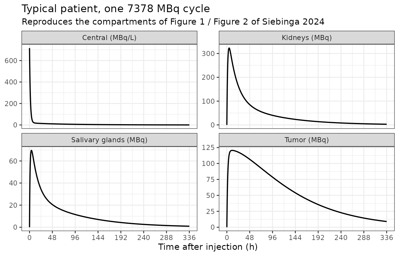
The cycle effect on tumor uptake
The paper’s headline PK finding is that tumor uptake declines over cycles, to 73%, 50% and 44% of the cycle-1 rate in cycles 2, 3 and 4-7 (Table 2, Equation 8). Reading the tumor uptake rate constant back out of the packaged model confirms the encoding.
cycle_check <- lapply(1:4, function(cy) {
  ev <- events_pk |> mutate(CYCLE = cy)
  rxode2::rxSolve(mod_typical, events = ev, useLinCmt = FALSE) |>
    as.data.frame() |>
    summarise(cycle = cy, kin_tumor = first(kin_tumor))
}) |>
  bind_rows() |>
  mutate(
    fraction_of_cycle1 = kin_tumor / kin_tumor[cycle == 1],
    published = c(1, 0.731, 0.498, 0.436)
  )
#> ℹ omega/sigma items treated as zero: 'etalkel', 'etalkin_kidney', 'etalkin_tumor', 'etalkin_other', 'etalbmax', 'etarbase', 'etalkgrow', 'etalkd_direct', 'etalkd_delay', 'etaiov_kin_tumor_1', 'etaiov_kin_tumor_2', 'etaiov_kin_tumor_3', 'etaiov_kin_tumor_4', 'etaiov_kin_tumor_5', 'etaiov_kin_tumor_6', 'etaiov_kin_tumor_7', 'etaiov_kin_tumor_8'
#> ℹ omega/sigma items treated as zero: 'etalkel', 'etalkin_kidney', 'etalkin_tumor', 'etalkin_other', 'etalbmax', 'etarbase', 'etalkgrow', 'etalkd_direct', 'etalkd_delay', 'etaiov_kin_tumor_1', 'etaiov_kin_tumor_2', 'etaiov_kin_tumor_3', 'etaiov_kin_tumor_4', 'etaiov_kin_tumor_5', 'etaiov_kin_tumor_6', 'etaiov_kin_tumor_7', 'etaiov_kin_tumor_8'
#> ℹ omega/sigma items treated as zero: 'etalkel', 'etalkin_kidney', 'etalkin_tumor', 'etalkin_other', 'etalbmax', 'etarbase', 'etalkgrow', 'etalkd_direct', 'etalkd_delay', 'etaiov_kin_tumor_1', 'etaiov_kin_tumor_2', 'etaiov_kin_tumor_3', 'etaiov_kin_tumor_4', 'etaiov_kin_tumor_5', 'etaiov_kin_tumor_6', 'etaiov_kin_tumor_7', 'etaiov_kin_tumor_8'
#> ℹ omega/sigma items treated as zero: 'etalkel', 'etalkin_kidney', 'etalkin_tumor', 'etalkin_other', 'etalbmax', 'etarbase', 'etalkgrow', 'etalkd_direct', 'etalkd_delay', 'etaiov_kin_tumor_1', 'etaiov_kin_tumor_2', 'etaiov_kin_tumor_3', 'etaiov_kin_tumor_4', 'etaiov_kin_tumor_5', 'etaiov_kin_tumor_6', 'etaiov_kin_tumor_7', 'etaiov_kin_tumor_8'

cycle_check |>
  dplyr::rename("Cycle" = cycle, "kin_tumor (1/h)" = kin_tumor,
                "Fraction of cycle 1" = fraction_of_cycle1,
                "Published fraction (Table 2)" = published) |>
  knitr::kable(digits = 5,
caption = "Structural cycle effect on the tumor uptake rate constant.")| Cycle | kin_tumor (1/h) | Fraction of cycle 1 | Published fraction (Table 2) |
|---|---|---|---|
| 1 | 0.00967 | 1.000 | 1.000 |
| 2 | 0.00707 | 0.731 | 0.731 |
| 3 | 0.00482 | 0.498 | 0.498 |
| 4 | 0.00422 | 0.436 | 0.436 |
Structural effect of tumor volume on tumor uptake
The paper states that “a two-times higher volume resulted in a 2.11-fold increased tumor uptake rate” (Results), which is the power exponent 1.08.
two_fold <- vapply(c(44300, 88600), function(tv) {
  ev <- events_pk |> mutate(TUM_VOL = tv)
  rxode2::rxSolve(mod_typical, events = ev, useLinCmt = FALSE) |>
    as.data.frame() |>
    (\(d) d$kin_tumor[1])()
}, numeric(1))
#> ℹ omega/sigma items treated as zero: 'etalkel', 'etalkin_kidney', 'etalkin_tumor', 'etalkin_other', 'etalbmax', 'etarbase', 'etalkgrow', 'etalkd_direct', 'etalkd_delay', 'etaiov_kin_tumor_1', 'etaiov_kin_tumor_2', 'etaiov_kin_tumor_3', 'etaiov_kin_tumor_4', 'etaiov_kin_tumor_5', 'etaiov_kin_tumor_6', 'etaiov_kin_tumor_7', 'etaiov_kin_tumor_8'
#> ℹ omega/sigma items treated as zero: 'etalkel', 'etalkin_kidney', 'etalkin_tumor', 'etalkin_other', 'etalbmax', 'etarbase', 'etalkgrow', 'etalkd_direct', 'etalkd_delay', 'etaiov_kin_tumor_1', 'etaiov_kin_tumor_2', 'etaiov_kin_tumor_3', 'etaiov_kin_tumor_4', 'etaiov_kin_tumor_5', 'etaiov_kin_tumor_6', 'etaiov_kin_tumor_7', 'etaiov_kin_tumor_8'

cat(sprintf("Doubling tumor volume multiplies kin_tumor by %.3f (paper: 2.11)\n",
            two_fold[2] / two_fold[1]))
#> Doubling tumor volume multiplies kin_tumor by 2.114 (paper: 2.11)
stopifnot(abs(two_fold[2] / two_fold[1] - 2^1.08) < 1e-6)
Figure 5 – simulated PSA dynamics for the two dosing regimens
The paper plots the median simulated PSA with a 50% prediction interval for both schedules and observes “only slight differences”, with the “2 x 2 - repeated” arm showing a more prominent decrease just after the second cycle.
psa_summary <- sim_pd |>
  group_by(regimen, time) |>
  summarise(
    median = stats::median(PSA),
    lo = stats::quantile(PSA, 0.25),
    hi = stats::quantile(PSA, 0.75),
    .groups = "drop"
  )

ggplot(psa_summary, aes(time / week, median, fill = regimen, colour = regimen)) +
  geom_ribbon(aes(ymin = lo, ymax = hi), alpha = 0.2, colour = NA) +
  geom_line(linewidth = 0.8) +
  geom_vline(xintercept = 24, linetype = "dashed", linewidth = 0.3) +
  scale_x_continuous(breaks = seq(0, 32, by = 4)) +
  labs(x = "Time after start of treatment (weeks)", y = "PSA (ug/L)",
       colour = "Regimen", fill = "Regimen",
       title = "Simulated PSA dynamics (median and 50% prediction interval)",
       subtitle = "Replicates Figure 5 of Siebinga 2024; dashed line is the 24-week response endpoint") +
  theme_bw() + theme(legend.position = "top")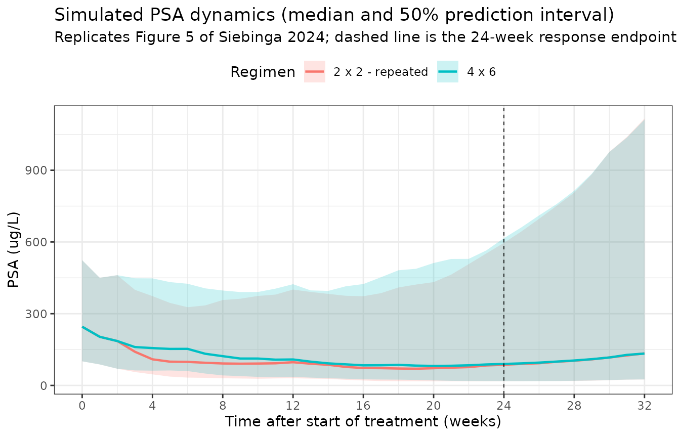
Simulated response rates
The paper’s quantitative simulation endpoints (Results, “Simulations”): response is a >= 50% decrease in PSA at 24 weeks and stable disease is no increase in PSA at 24 weeks.
response <- sim_pd |>
  filter(time %in% c(0, 24 * week)) |>
  select(regimen, id, time, PSA) |>
  tidyr::pivot_wider(names_from = time, values_from = PSA,
                     names_prefix = "t") |>
  mutate(change = (.data[[paste0("t", 24 * week)]] - t0) / t0) |>
  group_by(regimen) |>
  summarise(
    response = 100 * mean(change <= -0.5),
    stable = 100 * mean(change <= 0),
    .groups = "drop"
  ) |>
  mutate(
    published_response = c(42.4, 44.7)[match(regimen, c("4 x 6", "2 x 2 - repeated"))],
    published_stable = c(54.8, 56.4)[match(regimen, c("4 x 6", "2 x 2 - repeated"))]
  )

response |>
  dplyr::rename(
    "Regimen" = regimen,
    "Response, simulated (%)" = response,
    "Stable disease, simulated (%)" = stable,
    "Response, published (%)" = published_response,
    "Stable disease, published (%)" = published_stable
  ) |>
  knitr::kable(digits = 1,
caption = "Treatment response at 24 weeks vs. the published simulation (n = 2000 in the paper, 200 per arm here).")| Regimen | Response, simulated (%) | Stable disease, simulated (%) | Response, published (%) | Stable disease, published (%) |
|---|---|---|---|---|
| 2 x 2 - repeated | 46.5 | 61.0 | 44.7 | 56.4 |
| 4 x 6 | 46.0 | 60.5 | 42.4 | 54.8 |
Both proportions land within a few percentage points of the published values, and the ordering (the “2 x 2 - repeated” arm slightly ahead) is reproduced. The residual gap is consistent with the smaller cohort and with the covariate distributions being reconstructed from medians and ranges rather than from the original patient-level data.
PKNCA validation
Two NCA passes. The first is a conventional NCA of the central-compartment activity concentration, whose clearance is directly comparable to the renal clearance the paper quotes. The second integrates the tumor activity concentration to the cumulative tumor exposure that the paper’s threshold analysis uses.
conc_central <- sim_pk |>
  filter(!is.na(Cc)) |>
  select(id, time, Cc) |>
  mutate(treatment = "7378 MBq single cycle")

conc_central <- bind_rows(
  conc_central,
  conc_central |> distinct(id, treatment) |> mutate(time = 0, Cc = 0)
) |>
  distinct(id, treatment, time, .keep_all = TRUE) |>
  arrange(id, treatment, time)

dose_obj <- PKNCA::PKNCAdose(
  events_pk |> filter(evid == 1L) |>
    transmute(id, time, amt, treatment = "7378 MBq single cycle"),
  amt ~ time | treatment + id
)

nca_central <- PKNCA::pk.nca(PKNCA::PKNCAdata(
  PKNCA::PKNCAconc(conc_central, Cc ~ time | treatment + id),
  dose_obj,
  intervals = data.frame(start = 0, end = Inf, cmax = TRUE, tmax = TRUE,
                         aucinf.obs = TRUE, cl.obs = TRUE, half.life = TRUE)
))

nca_central_df <- as.data.frame(nca_central) |>
  filter(PPTESTCD %in% c("cmax", "tmax", "aucinf.obs", "cl.obs", "half.life"))

nca_central_df |>
  select(PPTESTCD, PPORRES) |>
  dplyr::rename("NCA parameter" = PPTESTCD, "Simulated" = PPORRES) |>
  knitr::kable(digits = 3,
caption = "NCA of the simulated central-compartment activity concentration (typical patient).")| NCA parameter | Simulated |
|---|---|
| cmax | 716.311 |
| tmax | 0.000 |
| half.life | 64.066 |
| aucinf.obs | 2831.614 |
| cl.obs | 2.606 |
conc_tumor <- sim_pk |>
  filter(!is.na(Ctumor)) |>
  select(id, time, Ctumor) |>
  mutate(treatment = "7378 MBq single cycle")

conc_tumor <- bind_rows(
  conc_tumor,
  conc_tumor |> distinct(id, treatment) |> mutate(time = 0, Ctumor = 0)
) |>
  distinct(id, treatment, time, .keep_all = TRUE) |>
  arrange(id, treatment, time)

nca_tumor <- PKNCA::pk.nca(PKNCA::PKNCAdata(
  PKNCA::PKNCAconc(conc_tumor, Ctumor ~ time | treatment + id),
  dose_obj,
  intervals = data.frame(start = 0, end = 1008, auclast = TRUE, cmax = TRUE)
))

tumor_auc_cycle1 <- as.data.frame(nca_tumor) |>
  filter(PPTESTCD == "auclast") |>
  pull(PPORRES)

# The paper's threshold is the cumulative tumor AUC of the FIRST TWO cycles;
# cycle 2 carries the 0.731 uptake fraction of Table 2.
two_cycle_auc_mbq_h_per_ml <- tumor_auc_cycle1 * (1 + 0.731) / 1000

cat(sprintf(
  "Typical-patient tumor AUC, cycles 1+2: %.0f MBq*h/mL\nPublished response thresholds: 709.5 (nadir PSA) and 1188 (last PSA)\n",
  two_cycle_auc_mbq_h_per_ml))
#> Typical-patient tumor AUC, cycles 1+2: 735 MBq*h/mL
#> Published response thresholds: 709.5 (nadir PSA) and 1188 (last PSA)
The typical (median-tumor-volume, median-weight, no-random-effects)
patient lands between the paper’s two published
thresholds: just above the 709.5 MBqh/mL required for a
>= 50% decrease at the PSA nadir, and well below the 1188
MBqh/mL required for a >= 50% decrease at the last
measurement after two cycles. That is the expected placement. The
published response rate at the later, stricter endpoint is 42-45%, so
the median patient should fall short of it, while a majority transiently
reach a 50% decrease at nadir. Whether an individual clears either
threshold is driven by the tumor-uptake random effects (IIV 63.4% CV
plus IOV 37.8% CV on kin_tumor).
stopifnot(
  two_cycle_auc_mbq_h_per_ml > 709.5,
  two_cycle_auc_mbq_h_per_ml < 1188
)
Comparison against published values
The paper reports no plasma NCA table, but the Discussion gives three derived quantities that the NCA above reproduces directly, plus the tumor half-life.
The clearance of the central compartment is the one NCA parameter the
paper states outright: “Renal clearance was estimated 2.61 L/h”
(Discussion). Because renal excretion via k10 is the
model’s only route of elimination, the NCA-derived clearance must equal
k10 * V1 exactly, which makes this a sharp check on the
encoded lkel and lvc.
cmp <- nlmixr2lib::ncaComparisonTable(
  simulated = data.frame(
    PPTESTCD = "cl.obs",
    PPORRES = nca_central_df$PPORRES[nca_central_df$PPTESTCD == "cl.obs"]
  ),
  reference = data.frame(cl.obs = 2.61),
  units = c(cl.obs = "L/h"),
  tolerance_pct = 20
)

knitr::kable(cmp, digits = 3,
             caption = paste("Simulated central-compartment clearance vs. the",
                             "renal clearance quoted in the Discussion of",
"Siebinga 2024."))| NCA parameter | Reference | Simulated | % diff |
|---|---|---|---|
| CL/F (L/h) | 2.61 | 2.61 | -0.2% |
The terminal half-life returned by the NCA above is not
log(2) / k10: the slowest eigenvalue of the
five-compartment system is the tumor efflux (k41 = 0.0150
1/h), so the central-compartment profile decays with the tumor
compartment in its terminal phase. The compartment-specific half-lives
the paper quotes are the individual efflux rate constants, tabulated
next.
tibble::tibble(
  Quantity = c("Organs at risk (salivary gland, k21)",
               "Organs at risk (kidney, k31)",
               "Tumor (k41)",
               "PSA growth rate kG (1/h)"),
  Model = c(log(2) / 0.0629, log(2) / 0.0625, log(2) / 0.0150, 0.000408),
  Published = c(11, 11, 46, 0.000408),
  `Published comparator` = c("~11 h (Discussion)", "~11 h (Discussion)",
                             "~46 h (Discussion)",
                             "0.000366 1/h in castration-resistant PCa (van Hasselt 2015)")
) |>
  knitr::kable(digits = 4,
caption = "Structural half-lives and the PSA growth rate against the values quoted in the Discussion.")| Quantity | Model | Published | Published comparator |
|---|---|---|---|
| Organs at risk (salivary gland, k21) | 11.0198 | 11.0000 | ~11 h (Discussion) |
| Organs at risk (kidney, k31) | 11.0904 | 11.0000 | ~11 h (Discussion) |
| Tumor (k41) | 46.2098 | 46.0000 | ~46 h (Discussion) |
| PSA growth rate kG (1/h) | 0.0004 | 0.0004 | 0.000366 1/h in castration-resistant PCa (van Hasselt 2015) |
Assumptions and deviations
Errata and value conflicts in the source
-
kD,directis printed two ways. The Results text states “K D, direct was estimated 0.000335 Lday-1GBq-1 (40.1% RSE)” while Table 3 gives 0.00335 (40.1% RSE, 95% CI 0.000961-0.006147) – a factor of ten apart. Table 3 is used. Its three numbers are mutually consistent: an RSE of 40.1% on 0.00335 implies a 95% CI of roughly 0.00072-0.0060, which is the interval printed; the same RSE on 0.000335 would imply an interval ten times narrower than the one printed. The text value is inconsistent with the interval printed beside it. The choice is also low-impact: because the delayed effect integrates to roughly ten times the direct effect, the simulated 24-week response rate moves by only about five percentage points between the two readings, and both remain compatible with the published 42-45%. - The sign of the tumor-volume effect on salivary-gland uptake. The Results narrative says “an increased tumor volume resulted in a lower salivary gland uptake rate (k12)”, describing a tumor sink effect, but Table 2 prints the power exponent as +0.0910 with a 95% CI of 0.0350-0.544 that is entirely positive. Table 2 is used (a positive exponent), because the estimate, its RSE and the lower confidence bound all agree on the sign while the narrative is a single qualitative clause. The effect is weak either way: a ten-fold increase in tumor volume changes k12 by only 23%. Note also that the printed upper bound of 0.544 is not consistent with an RSE of 30.0%, which suggests a typographical error somewhere in that table row; the point estimate is unaffected.
-
Radioactive decay. Methods say the PD driver is
“the estimated concentration in the tumor compartment (taking into
account radioactive decay)”, while all radioactivity data were
“corrected for decay to the time of injection”. The model here takes the
states to be decay-corrected (as in the predecessor
Siebinga_2023_lu177psma617) and drives the PD directly from them, reading the parenthetical as a statement that decay was handled in the data correction. Encoding an additional explicit Lu-177 physical-decay term on every state was tested and rejected: it drops the simulated 24-week response rate to about 29% against the published 42-45%, far outside Monte-Carlo error, whereas the decay-corrected reading reproduces the published rates. This also keeps the model free of any constant not printed in the paper. - Supplement. Additional file 1 (individual model fit results, Figures S1-S4) was not available when this model was built. It contains individual prediction-vs-observation plots only; every parameter used here comes from Table 2, Table 3 or the Methods text, so nothing is missing from the extraction.
Modelling assumptions
-
Allometric scaling. Methods state that body weight
was scaled “in relation to the median body weight, where exponents for
volume of distribution (V) and rate constants (k) were set to 1 and
-0.25”. Both exponents are therefore encoded as
fixed(), and the reference is the Table 1 median of 79 kg (the paper does not restate the centering value).Bmaxis neither a volume nor a rate constant and the sentence names only V and k, soBmaxis left unscaled. - Covariate reference values. The paper’s covariate equations are all normalised to “the median value of the tested covariate” without restating it, so the Table 1 medians are used throughout: 79 kg for weight and 0.0443 L (44300 mm^3) for segmented tumor volume.
-
Interoccasion variability. nlmixr2 has no
equivalent of NONMEM’s
$OMEGA BLOCK(1) SAME, so occasions 2-8 each carry their own eta with the variance fixed equal to the estimated occasion-1 variance. Eight occasions cover the maximum number of cycles in Table 1. -
Box-Cox transformed eta. The IIV on
kGwas Box-Cox transformed by the authors (Table 3 shape parameter -0.822). It is implemented inmodel()in the standard Petersson form,phi = (exp(eta)^lambda - 1) / lambdafollowed bykG = kG_pop * exp(phi), because rxode2’sboxCox()applies to residual error rather than to etas. The reported 90.9% CV is taken to be the variance of the untransformed eta, which is what NONMEM reports in$OMEGA. -
Cycle counting.
CYCLEis a time-varying covariate that counts administrations. It carries both the structural Equation 8 cycle effect and the interoccasion-variability occasion index, and is decomposed into binary indicators insidemodel()rather than entering any equation as an integer. - Covariate distributions for the simulation. The paper simulated 2000 patients from “patient characteristic distributions of all included covariates” but does not publish those distributions. Weight is drawn normally and tumor volume log-normally, both matched to the Table 1 median and truncated to the Table 1 range. The simulated response rates are therefore expected to differ from the published ones by a few percentage points.
-
Screened but unused covariates. Creatinine
clearance (on
k10) and age (on baseline PSA) were tested and not retained, and no coefficients are published for them; hematocrit is reported in Table 1 but never tested. All three are recorded incovariatesDataExcludedrather thancovariateData. -
Cycle effects on the salivary gland. The Discussion
mentions a cycle effect on salivary-gland uptake (84.6% in cycle 2,
98.1% in cycle 3), but Table 2 lists cycle effects only on
k14, so the final model carries none onk12and neither does this encoding.