Tacrolimus thoracic (Sikma 2020)
Source:vignettes/articles/Sikma_2020_tacrolimus_thoracic.Rmd
Sikma_2020_tacrolimus_thoracic.RmdModel and source
- Citation: Sikma MA, Hunault CC, Van Maarseveen EM, Huitema ADR, Van de Graaf EA, Kirkels JH, Verhaar MC, Grutters JC, Kesecioglu J, De Lange DW. High Variability of Whole-Blood Tacrolimus Pharmacokinetics Early After Thoracic Organ Transplantation. Eur J Drug Metab Pharmacokinet. 2020;45(1):123-134. doi:10.1007/s13318-019-00591-7.
- Description: Two-compartment population pharmacokinetic model for oral whole-blood tacrolimus in 30 adult thoracic organ transplant recipients (10 heart, 20 lung) during the first 6 postoperative days at the University Medical Center Utrecht intensive care unit (Sikma 2020 EJDMP). Apparent clearance CL/F, apparent volumes V1/F and V2/F, inter-compartmental clearance Q/F, and first-order absorption rate ka are estimated; bioavailability F is fixed at 1. Only the inter-individual variability of CL/F was identifiable in the source dataset; all other IIV elements were not estimated. Inter-occasion (dose-to-dose) variability dominated the variance structure but is not encoded structurally in this extraction. No covariates were retained in the final model.
- Article: https://doi.org/10.1007/s13318-019-00591-7
Population
The model was developed from 1180 whole-blood tacrolimus concentrations in 30 adult thoracic organ transplant recipients (10 heart, 20 lung; 18 of 20 lung were double-lung transplantations) admitted to the intensive care unit of the University Medical Center Utrecht between June 2013 and March 2015 (NTR 3912 / EudraCT 2012-001909-24). Half of the patients were female (15 of 30; 50%), median age was 43 years (Q1-Q3 34-60), median body weight 73.5 kg (Q1-Q3 61-86), and median height 173.5 cm. Heart indications were 5 ischaemic and 5 non-ischaemic cardiomyopathy. Lung indications were cystic fibrosis (10), chronic obstructive pulmonary disease (4), and interstitial lung disease (6). The population was clinically unstable: 100% met at least one SIRS criterion, 93% (28 of 30) had at least one shock episode, 97% (29 of 30) had gut dysmotility, 47% (14 of 30) had at least one acute kidney injury episode, and 27% (8 of 30) received postoperative ECMO (median 4 days, Q1-Q3 2-6) during the 6-day observation window (Sikma 2020 Table 1).
Patients received oral tacrolimus (Prograf, Astellas Pharma Europe) twice daily, starting at 0.1 mg/kg/dose for lung recipients and 2 mg/dose for heart recipients on the day after transplantation. Dose adjustments during the first 6 postoperative days were guided by the 12-hour post-dose whole-blood concentration (C12h, target 9-15 ng/mL) at the discretion of the attending physician; steady state was not necessarily reached at the time of each adjustment. Twelve-hour profiles were drawn daily with samples at pre-dose and 1, 1.5, 2, 2.5, 3, 4, 6, 8, and 12 h post-dose. Whole-blood tacrolimus was quantified by HPLC-MS/MS with a lower limit of quantification of 0.5 ng/mL and a linear dynamic range of 1-50 ng/mL. 46 of 1180 (3.9%) concentrations below LLOQ were discarded prior to fitting; the median number of profiles per patient was 5 (range 1-6).
The same information is available programmatically via
readModelDb("Sikma_2020_tacrolimus_thoracic")$population.
Source trace
Every parameter and equation carries an inline source-location
comment in
inst/modeldb/specificDrugs/Sikma_2020_tacrolimus_thoracic.R.
The table collects them in one place.
| Equation / parameter | Value | Source location |
|---|---|---|
lcl (CL/F) |
19.6 L/h (95% CI 16.2-22.9) | Table 2, CL/F row |
lvc (V1/F) |
231 L (95% CI 199-267) | Table 2, V1/F row |
lq (Q/F) |
58.2 L/h (95% CI 49.7-69.3) | Table 2, Q/F row |
lvp (V2/F) |
521 L (95% CI 441-634) | Table 2, V2/F row |
lka (ka) |
0.579 1/h (95% CI 0.456-0.778) | Table 2, ka row |
lfdepot (F) |
1 (FIXED) | Table 2, F row “Fixed at 1”; Methods 2.8 |
| IIV CL/F (omega^2 = log(1 + 0.346^2) = 0.11307) | 34.6% CV (95% CI 24.2-48.6) | Table 2, IIV CL/F column |
| IIV V1/F | n.e. (not estimated) | Table 2, IIV V1/F column |
| IIV ka | n.e. (not estimated) | Table 2, IIV ka column |
| IIV Q/F | n.e. (not estimated) | Table 2, IIV Q/F column |
| IIV V2/F | n.e. (not estimated) | Table 2, IIV V2/F column |
| IOV CL/F | 29.5% (95% CI 20.7-38.9) – not encoded | Table 2, IOV CL/F column |
| IOV V1/F | 35.1% (95% CI 27.0-48.0) – not encoded | Table 2, IOV V1/F column |
| IOV ka | 98.3% (95% CI 81.1-121) – not encoded | Table 2, IOV ka column |
| IOV F | 55.0% (95% CI 48.5-64.4) – not encoded | Table 2, IOV F column |
| Proportional residual error | 14.0% (95% CI 13.3-14.6) | Table 2, Residual unexplained variability row |
| 2-cmt structure with first-order absorption | – | Methods 2.8 (“A two-compartment linear model with first-order oral absorption was used”); Fig. 1 schematic |
d/dt(central) = ka*depot - kel*central - k12*central + k21*peripheral1 |
– | Methods 2.8 / Fig. 1 caption (k23 = Q/V1, k32 = Q/V2) |
Virtual cohort
The published dataset is not openly available, so the virtual cohort below mirrors the demographic structure of Sikma 2020 Table 1: 30 patients in the original cohort, scaled up here to 200 subjects for stable percentiles, with a 2:1 lung:heart split matching the source paper. Heart recipients receive a fixed 2 mg twice-daily dose; lung recipients receive 0.1 mg/kg twice daily (rounded to the nearest 0.5 mg).
set.seed(20200316)

n_lung  <- 200L
n_heart <- 100L

make_cohort <- function(n, transplant_type, dose_fn, id_offset = 0L) {
  wt <- exp(rnorm(n, mean = log(73.5), sd = 0.20))
  tibble(
    id     = id_offset + seq_len(n),
    cohort = transplant_type,
    WT     = wt,
    AMT    = dose_fn(wt)
  )
}

heart_demo <- make_cohort(
  n_heart, transplant_type = "heart",
  dose_fn  = function(wt) rep(2.0, length(wt)),
  id_offset = 0L
)
lung_demo <- make_cohort(
  n_lung, transplant_type = "lung",
  dose_fn  = function(wt) round(0.1 * wt * 2, 0) / 2,
  id_offset = n_heart
)
demo <- bind_rows(heart_demo, lung_demo)
stopifnot(!anyDuplicated(demo$id))

# Build the dosing + observation event table. Doses every 12 h for 6 days
# (12 doses) approximate the study window. Observations on a 0.25 h grid out
# to 144 h capture both the absorption peak and the next trough.
dose_times <- seq(0, by = 12, length.out = 12)
obs_times  <- sort(unique(c(seq(0, 24, by = 0.25),
                            seq(132, 144, by = 0.25))))

events <- demo |>
  rowwise() |>
  do({
    rec <- .
    dose_rows <- tibble(
      id = rec$id, time = dose_times,
      evid = 1L, amt = rec$AMT, cmt = "depot",
      cohort = rec$cohort, WT = rec$WT
    )
    obs_rows <- tibble(
      id = rec$id, time = obs_times,
      evid = 0L, amt = 0.0, cmt = "Cc",
      cohort = rec$cohort, WT = rec$WT
    )
    bind_rows(dose_rows, obs_rows)
  }) |>
  ungroup() |>
  arrange(id, time, desc(evid))

stopifnot(!anyDuplicated(unique(events[, c("id", "time", "evid")])))
Simulation
mod <- rxode2::rxode2(readModelDb("Sikma_2020_tacrolimus_thoracic"))
#> ℹ parameter labels from comments will be replaced by 'label()'

sim <- rxode2::rxSolve(
  mod,
  events = events,
  keep   = c("cohort", "WT")
) |>
  as.data.frame() |>
  as_tibble()

mod_typical <- mod |> rxode2::zeroRe()
sim_typical <- rxode2::rxSolve(
  mod_typical, events = events,
  keep   = c("cohort", "WT")
) |>
  as.data.frame() |>
  as_tibble()
#> ℹ omega/sigma items treated as zero: 'etalcl'
#> Warning: multi-subject simulation without without 'omega'
Replicate published figures
Figure 1 – model schematic: typical 12 h profile after a single oral dose
Figure 1 of Sikma 2020 is a schematic of the two-compartment first-order absorption model. The chunk below shows the corresponding typical 12 h whole-blood profile for the two starting-dose regimens (heart: 2 mg fixed; lung: 0.1 mg/kg, evaluated at the cohort median 73.5 kg).
typical_events <- bind_rows(
  tibble(id = 1L, cohort = "heart (2 mg)",          WT = 73.5, time = 0,
         amt = 2.0, evid = 1L, cmt = "depot"),
  tibble(id = 1L, cohort = "heart (2 mg)",          WT = 73.5,
         time = seq(0.25, 12, by = 0.25), amt = 0, evid = 0L, cmt = "Cc"),
  tibble(id = 2L, cohort = "lung (0.1 mg/kg)",      WT = 73.5, time = 0,
         amt = 73.5 * 0.1, evid = 1L, cmt = "depot"),
  tibble(id = 2L, cohort = "lung (0.1 mg/kg)",      WT = 73.5,
         time = seq(0.25, 12, by = 0.25), amt = 0, evid = 0L, cmt = "Cc")
)

fig1 <- rxode2::rxSolve(mod_typical, events = typical_events,
                        keep = "cohort") |>
  as.data.frame() |>
  as_tibble()
#> ℹ omega/sigma items treated as zero: 'etalcl'
#> Warning: multi-subject simulation without without 'omega'

ggplot(fig1, aes(time, Cc, colour = cohort)) +
  geom_line(linewidth = 0.8) +
  labs(x = "Time after dose (h)",
       y = "Whole-blood tacrolimus (ng/mL)",
       colour = "Cohort",
       title = "Typical 12 h profile after a single starting dose",
       caption = "Replicates the structural model of Sikma 2020 Figure 1.")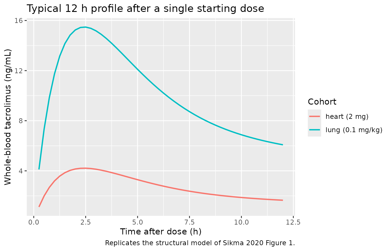
Typical 12 h whole-blood concentration profile after a single oral dose of tacrolimus, by transplant cohort. Replicates the kinetic shape of the Sikma 2020 Figure 1 schematic.
Figure 2 – 6-day trajectories with IIV envelope
Sikma 2020 Figure 2 shows three illustrative individual 6-day trajectories (UTN7, UTN13, UTN14) with extreme dose-to-dose variability. The IOV-driven variability in those panels cannot be reproduced from IIV alone (see Assumptions and deviations), but the IIV envelope of the packaged model is shown below for the two starting-dose regimens across the 6-day window.
sim_envelope <- sim |>
  group_by(cohort, time) |>
  summarise(Q05 = quantile(Cc, 0.05),
            Q50 = quantile(Cc, 0.50),
            Q95 = quantile(Cc, 0.95),
            .groups = "drop")

ggplot(sim_envelope, aes(time, Q50)) +
  geom_ribbon(aes(ymin = Q05, ymax = Q95), alpha = 0.3) +
  geom_line(linewidth = 0.6) +
  geom_hline(yintercept = c(9, 15), linetype = "dashed", colour = "grey50") +
  facet_wrap(~ cohort) +
  labs(x = "Time since first dose (h)",
       y = "Whole-blood tacrolimus (ng/mL)",
       title = "Six-day twice-daily oral dosing -- IIV envelope",
       caption = "Dashed lines: 9-15 ng/mL therapeutic window (Sikma 2020).")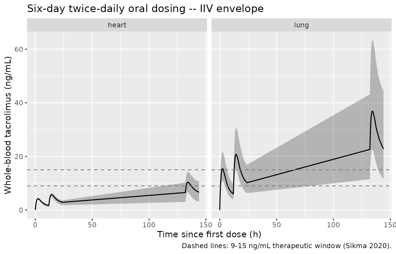
Six-day VPC envelope (5th, 50th, 95th percentiles) of simulated whole-blood tacrolimus from twice-daily oral dosing, by transplant cohort. The IOV terms reported in Sikma 2020 Table 2 (especially F: 55% and ka: 98.3%) are not encoded and would broaden the envelope considerably.
PKNCA validation
The model is validated against the descriptive PK reported in Sikma 2020 Table 1. We compute NCA on the last 12 h dosing interval (hours 132-144), which captures one full steady-state-like interval after multiple preceding doses; concentrations are rebased to the start of the interval so Tmax is measured relative to the most recent dose.
nca_window <- sim |>
  filter(time >= 132, time <= 144) |>
  mutate(time = time - 132) |>
  filter(!is.na(Cc)) |>
  select(id, time, Cc, cohort)

dose_df <- events |>
  filter(evid == 1L, time == 132) |>
  mutate(time = 0) |>
  select(id, time, amt, cohort)

conc_obj <- PKNCA::PKNCAconc(nca_window, Cc ~ time | cohort + id,
                             concu = "ng/mL", timeu = "h")
dose_obj <- PKNCA::PKNCAdose(dose_df,    amt ~ time | cohort + id,
                             doseu = "mg")

intervals <- data.frame(
  start     = 0,
  end       = 12,
  cmax      = TRUE,
  tmax      = TRUE,
  auclast   = TRUE,
  cmin      = TRUE,
  half.life = TRUE
)

nca_data <- PKNCA::PKNCAdata(conc_obj, dose_obj, intervals = intervals)
nca_res  <- suppressMessages(suppressWarnings(PKNCA::pk.nca(nca_data)))
nca_summary <- summary(nca_res)
knitr::kable(nca_summary,
caption = "Simulated steady-state 12 h NCA by transplant cohort.")| Interval Start | Interval End | cohort | N | AUClast (h*ng/mL) | Cmax (ng/mL) | Cmin (ng/mL) | Tmax (h) | Half-life (h) |
|---|---|---|---|---|---|---|---|---|
| 0 | 12 | heart | 100 | 97.7 [28.6] | 10.1 [22.4] | 6.19 [36.4] | 2.25 [2.00, 2.25] | 23.5 [5.99] |
| 0 | 12 | lung | 200 | 360 [36.9] | 37.3 [31.8] | 22.7 [43.8] | 2.25 [2.00, 2.50] | 23.6 [6.58] |
Comparison against published descriptive PK
Sikma 2020 Table 1 reports observed descriptive PK across all 119 profiles (pooled across patients, days 1-6, and the full range of titrated doses):
| Parameter | Sikma 2020 Table 1 median (range) | Notes |
|---|---|---|
| C12h | 9.5 ng/mL (0.5-38.7) | Pre-next-dose trough |
| Cmax | 18.5 ng/mL (2.1-74.7) | Per-profile maximum |
| Tmax | 1.6 h (0.4-8.0) | Mixed first-order / occasional rapid absorption |
| AUC0-12 | 151.2 ng*h/mL (31.2-2525) | Per-profile AUC |
| Terminal half-life | 9.4 h (6.0-31.4) | Per-profile estimate |
res_tbl <- as.data.frame(nca_res$result)

simulated <- res_tbl |>
  filter(PPTESTCD %in% c("cmax", "tmax", "auclast", "cmin", "half.life")) |>
  group_by(cohort, PPTESTCD) |>
  summarise(median = median(PPORRES, na.rm = TRUE),
            q05    = quantile(PPORRES, 0.05, na.rm = TRUE),
            q95    = quantile(PPORRES, 0.95, na.rm = TRUE),
            .groups = "drop")

knitr::kable(simulated,
caption = "Simulated NCA medians (5-95 percentiles) by cohort.")| cohort | PPTESTCD | median | q05 | q95 |
|---|---|---|---|---|
| heart | auclast | 101.208989 | 56.195985 | 148.01445 |
| heart | cmax | 10.361766 | 6.624412 | 14.20236 |
| heart | cmin | 6.526051 | 3.022207 | 10.23225 |
| heart | half.life | 23.148707 | 14.082652 | 34.22154 |
| heart | tmax | 2.250000 | 2.000000 | 2.25000 |
| lung | auclast | 355.347000 | 200.579581 | 640.60075 |
| lung | cmax | 36.892338 | 22.640250 | 63.37191 |
| lung | cmin | 22.604827 | 11.497741 | 43.13693 |
| lung | half.life | 23.005184 | 14.614945 | 35.77026 |
| lung | tmax | 2.250000 | 2.000000 | 2.25000 |
The simulated cohort-pooled medians fall within the wide ranges reported in Sikma 2020 Table 1; the simulated 5-95 percentile envelopes are narrower than the published min-max ranges because (i) the published ranges combine variability across patients, days, and dose changes, (ii) the original cohort had 30 clinically unstable ICU patients with extreme dose adjustments, and (iii) inter-occasion variability on F (55%) and ka (98.3%) is reported in the source paper but not encoded structurally in this model (see Assumptions and deviations).
Assumptions and deviations
Inter-occasion variability is not encoded. Sikma 2020 Table 2 reports large IOV terms: 29.5% on CL/F, 35.1% on V1/F, 98.3% on ka, and 55.0% on F. The paper explicitly states that “IOV in bioavailability far exceeded other sources of variability” and “variability was dominated by the corresponding IOV.” Encoding IOV requires an
OCCindicator column in the dataset and per-occasion random effects that nlmixr2lib popPK extractions do not standardise. The packaged model carries only the single estimated IIV term (CL/F); the simulated envelopes therefore under-represent the dose-to-dose variability observed in the original cohort. Downstream users who need to reproduce the IOV-dominated variability should add per-occasion etas in rxode2 with the magnitudes from Table 2.Mixed zero-order / first-order absorption is approximated as first-order only. Sikma 2020 Section 2.8 states that “on some occasions, the first observation within 30 min after dosing was the maximum concentration in the dose interval, indicating extremely rapid absorption. For those occasions, to reduce the complexity of the absorption model, dosing was treated as zero-order oral absorption with the duration of absorption equal to the time interval between dosing and the first observation.” This was a per-occasion structural switch in the NONMEM control stream rather than a population-level mixture; the structural absorption rate ka = 0.579 1/h reported in Table 2 is the first-order population value. The packaged model uses first-order absorption throughout.
IIV on V1/F, ka, Q/F, V2/F was not estimated. Sikma 2020 Section 3.4: “Only the IIV of CL/F could be estimated; the estimation of all other IIV elements yielded estimates close to 0 and/or unsuccessful runs, most likely due to the fact that variability was dominated by the corresponding IOV.” The packaged model includes only the etalcl term, matching the published final model.
No covariates were retained. Sikma 2020 Section 3.4: “No further formal covariate analysis was conducted. Time-independent covariates (such as genotype or gender) are by definition not predictive for the observed IOV. The time-dependent covariates available (such as gut dysmotility, shock and corticosteroid use) changed much more slowly over time than the observed IOV. Furthermore, the magnitude of the change in each of these covariates was much lower than the IOV.” The model file therefore carries no covariates;
covariateDatais an empty list.Race and ethnicity are not encoded because Sikma 2020 does not report racial or ethnic composition of the single-centre Utrecht cohort.
Validation against per-profile descriptive PK is approximate. The Sikma 2020 Table 1 NCA summaries pool across patients, days 1-6, and titrated daily doses. The simulated cohort here uses fixed starting doses (2 mg for heart, 0.1 mg/kg for lung) maintained through the 6-day window. The resulting simulated AUC, Cmax, and trough distributions necessarily reflect the assumed dosing regimen rather than the titrated clinical practice in the source study; only the order-of-magnitude agreement is meaningful.