TV-46000 long-acting subcutaneous risperidone (Perlstein 2025)
Source:vignettes/articles/Perlstein_2025_risperidone_tv46000.Rmd
Perlstein_2025_risperidone_tv46000.RmdModel and source
#> ℹ parameter labels from comments will be replaced by 'label()'Citation: Perlstein I, Merenlender Wagner A, Elgart A, Zandvliet AS, Hellmann F, Lin Y, van Maanen E, Plock N, Fauchet F, Singh R (2025). Population pharmacokinetic modeling of TV-46000, a risperidone long-acting subcutaneous antipsychotic for the treatment of patients with schizophrenia. Neurol Ther 14(3):829-848. doi:10.1007/s40120-025-00723-z. Structural starting point from Ivaturi V, Gopalakrishnan M, Gobburu JVS, et al. (2017) Br J Clin Pharmacol 83(7):1476-1498; doi:10.1111/bcp.13246; see modellib(‘Ivaturi_2017_RBP_7000’).
Description: Sequential parent-metabolite population PK model for TV-46000, a long-acting subcutaneous antipsychotic (LASCA) that combines risperidone with a copolymer-based delivery technology in a suspension given subcutaneously once monthly (q1m) or once every 2 months (q2m), in 692 healthy volunteers and adults with schizophrenia or schizoaffective disorder pooled from three phase 1 and two phase 3 studies (Perlstein 2025). The single subcutaneous depot empties by two parallel first-order release routes: a fast direct route with rate constant ka1 straight into the risperidone central compartment (the initial release from the subcutaneous depot, which brings the total active moiety above 10 ng/mL within 24 h), and a slow indirect route with rate constant ka2 into a five-compartment transit chain with rate constant ktr that delivers the remainder into central over the 28-day or 56-day dosing interval (the in situ depot). Risperidone is described by a one-compartment model with first-order elimination CL/F, and because the fraction metabolized FRMET is fixed to 1 the whole of that elimination flux forms the equipotent metabolite 9-hydroxyrisperidone (paliperidone), which is itself described by a one-compartment model with first-order elimination CLMO. The two analytes are summed into the total active moiety in risperidone-equivalent units, TAM = [risperidone] + [9-OH-risperidone] * 410/426, which is the definition the paper gives in its Introduction and the same molecular-weight correction the upstream Ivaturi 2017 model applies. Body mass index shifts the balance between the two release routes (lower BMI gives a faster direct route and a slower indirect route), a larger injection volume slows the direct route, and upper-arm rather than abdominal injection raises ka1 by 33 percent. Interindividual variability is exponential on ka1, ka2 (correlated with ka1), CL and CLMO, and the log-transformed-both-sides residual error is proportional on each analyte. The total active moiety TAM = risperidone + 9-hydroxyrisperidone is the clinically reported quantity, and dopamine D2-receptor occupancy D2RO is derived from it with the literature Emax model the authors applied in their simulations (Emax 100 percent, kd 10.1 ng/mL). The structural starting point was the RBP-7000 dual-absorption model of Ivaturi 2017; see modellib(‘Ivaturi_2017_RBP_7000’).
Supplement (Table S1, Figures S1-S3): https://doi.org/10.1007/s40120-025-00723-z
TV-46000 is a long-acting subcutaneous antipsychotic (LASCA): risperidone suspended in a copolymer-based delivery vehicle at roughly 360 mg/mL and injected subcutaneously into the abdomen or the back of the upper arm once monthly (q1m) or once every 2 months (q2m). Perlstein 2025 pooled three phase 1 studies with the two phase 3 trials RISE and SHINE and fitted a sequential parent-metabolite population PK model: risperidone first, then 9-hydroxyrisperidone (paliperidone) driven by the parent’s individual post-hoc predictions.
The clinically reported quantity is the total active moiety (TAM), because risperidone and 9-hydroxyrisperidone are equipotent at the dopamine D2 receptor. Perlstein 2025 defines it in the Introduction as the “sum of concentrations of risperidone and its active metabolite [9-OH risperidone] corrected by molecular weight”, i.e. in risperidone-equivalent units.
Three risperidone models were already in the library when this one was added, and the contrast is worth stating because it decides which one a user should reach for:
-
modellib("Ivaturi_2017_RBP_7000")– the structural ancestor of this model. Perlstein 2025 Methods: “The starting point of the current analysis was the model reported by Ivaturi et al., which described sc absorption by one depot dose and a double first-order absorption route.” Ivaturi 2017 is a different LAI product (RBP-7000 / Atrigel) and pairs its PK with a PANSS exposure-response model. -
modellib("Wang_2024_risperidone_consta")andmodellib("Wang_2024_risperidone_rykindo")– intramuscular LAI formulations modelled on the active moiety directly, without splitting parent from metabolite. -
modellib("Feng_2008_risperidone"),modellib("Sherwin_2012_risperidone")– oral risperidone.
Population
The analysis dataset comprised 692 participants with at least one measurable plasma concentration after a TV-46000 injection: 267 from three phase 1 studies (50 healthy volunteers in RISPE1ZG15EU, 97 in SAD-10055, 120 in BA-10148) and 425 from the two phase 3 trials (352 in RISE, NCT03503318; 73 in SHINE, NCT03893825). Two further participants were excluded for self-administration of risperidone and 41 because every PK sample was below the limit of quantification (Perlstein 2025 Results “Dataset” and Table S1).
Baseline demographics (Perlstein 2025 Table 2, Total Overall column, n = 733 participants with baseline data) were: mean age 47.4 years (SD 10.9, range 16-65), 70.4% male, 64.7% Black or African American / 31.9% White / 1.4% Asian, mean weight 86.3 kg (SD 16.3, range 42-132), mean BMI 28.7 kg/m^2 (SD 4.8, range 18-38) and mean creatinine clearance 121 mL/min (SD 34.3). Across 3287 injections, 68.5% were abdominal and 31.5% into the upper arm, and 77.8% were delivered from a vial versus 22.2% from a prefilled syringe. The mean injection volume was 0.303 mL (SD 0.144).
Patients over 65 years were excluded from the source trials, and the Discussion flags the male and Black/African American skew as the analysis’s main generalizability limitation.
The same information is available programmatically:
str(readModelDb("Perlstein_2025_risperidone_tv46000")()$population, max.level = 1)
#> List of 14
#>  $ species       : chr "human"
#>  $ n_subjects    : int 692
#>  $ n_studies     : int 5
#>  $ n_observations: chr "Not reported as a record count. 692 participants contributed at least one measurable post-TV-46000 plasma conce"| __truncated__
#>  $ age_range     : chr "16-65 years; mean 47.4 (SD 10.9) years (Perlstein 2025 Table 2, Total Overall column). Patients older than 65 y"| __truncated__
#>  $ weight_range  : chr "42-132 kg; mean 86.3 (SD 16.3) kg (Perlstein 2025 Table 2)"
#>  $ bmi_range     : chr "18-38 kg/m^2; mean 28.7 (SD 4.8) kg/m^2 (Perlstein 2025 Table 2)"
#>  $ sex_female_pct: num 29.6
#>  $ race_ethnicity: Named num [1:4] 64.7 31.9 1.4 2
#>   ..- attr(*, "names")= chr [1:4] "Black" "White" "Asian" "Missing"
#>  $ renal_function: chr "Creatinine clearance mean 121 mL/min (SD 34.3); not reported for the healthy-volunteer study RISPE1ZG15EU (Perl"| __truncated__
#>  $ disease_state : chr "Adults with schizophrenia or schizoaffective disorder, plus 50 healthy volunteers (7.2% of the analysis populat"| __truncated__
#>  $ dose_range    : chr "TV-46000 subcutaneous. Phase 1: single doses 12.5-25 mg (RISPE1ZG15EU, subtherapeutic, healthy volunteers), sin"| __truncated__
#>  $ regions       : chr "Not reported by region; the phase 3 trials RISE (NCT03503318) and SHINE (NCT03893825) were multicenter"
#>  $ notes         : chr "Perlstein 2025 Table 2 tabulates demographics for the 733 participants with baseline data, while the popPK anal"| __truncated__
Source trace
Every ini() entry in
inst/modeldb/specificDrugs/Perlstein_2025_risperidone_tv46000.R
carries an in-file comment naming its source location. They are
collected here for review.
| Equation / parameter | Value | Source location |
|---|---|---|
Model structure (depot with parallel ka1 /
ka2 exits, 5-compartment ktr transit chain,
parent -> metabolite) |
n/a | Figure 1 (model schematic); Results, “Risperidone (Parent) PK Model” |
Continuous covariate form
Pi = P * (COVi / COVmedian)^theta_i
|
n/a | Methods, “Population PK Model Development” |
Categorical covariate form
Pi = P * (1 + theta_i)^COVi
|
n/a | Methods, “Population PK Model Development” |
lcl (CL/F) |
14.3 L/h | Table 3, risperidone (parent) |
lvc (V/F) |
66.3 L | Table 3, risperidone (parent) |
lka1 (KA1) |
0.000632 1/h | Table 3, risperidone (parent) |
lka2 (KA2) |
0.000408 1/h | Table 3, risperidone (parent) |
lktr (KTR) |
0.0252 1/h | Table 3, risperidone (parent) |
e_bmi_ka1 (KA1BMI1) |
-1.1 | Table 3 |
e_dose_ka1 (KA1INJV1) |
-0.384 | Table 3 |
e_injsite_arm_ka1 (KA1ADMSITE1) |
0.331 | Table 3; Results (“33% higher KA1” in the upper arm) |
e_bmi_ka2 (KA2BMI1) |
1.7 | Table 3 |
lcl_9oh (CLMO) |
5.78 L/h | Table 3, 9-OH risperidone (metabolite) |
lvc_9oh (VMO) |
95.7 L | Table 3, 9-OH risperidone (metabolite) |
| FRMET fixed to 1 | 1 | Table 3 footnote |
etalka2 / etalka1 block |
254.2% / 51.0% CV, correlation 42.8% | Table 3, random effects |
etalcl |
82.3% CV | Table 3, random effects |
etalcl_9oh |
65.1% CV | Table 3, random effects |
propSd (parent EP) |
40.5% | Table 3, residual error; Methods (log-transformed both sides) |
propSd_9oh (metabolite EP) |
38.3% | Table 3, residual error |
lemax (D2RO Emax) |
100% | Methods, “Prediction of Individual Exposure Parameters…” |
kd (D2RO) |
10.1 ng/mL | Methods, “Prediction of Individual Exposure Parameters…” |
| TAM = risperidone + molecular-weight-corrected 9-OH-risperidone | 410/426 | Introduction (definition of TAM); the two molecular weights are not printed – see Assumptions |
| Injection volumes 0.035 / 0.07 / 0.139 mL at 12.5 / 25 / 50 mg | n/a | Results, “Risperidone (Parent) PK Model”; 0.278 mL at 100 mg from Table 2 (BA-10148) |
| 28-day month for simulations | n/a | Methods, “Model-Based PK Simulations … for Different Dosing Regimens” |
Reading the IIV percentages
Table 3 reports each interindividual variability as a bare
percentage. Two conventions are in circulation –
%CV = 100 * sqrt(exp(omega^2) - 1) and the approximation
%CV = 100 * omega – and they disagree badly for the very
large KA2 term (omega^2 = 2.010 versus 6.462). The table’s
own confidence intervals settle it. Propagating the printed
%RSE as a relative standard error on
omega through the first (exact-lognormal)
transform reproduces the printed 95% CIs closely, while the second does
not:
| Parameter | Published %CV (95% CI) | omega^2 if lognormal | CI implied, lognormal | CI implied, omega=CV |
|---|---|---|---|---|
| KA2 | 254.2 (198.8-320.1) | 2.010 | 200.7-322.0 | 229.6-281.5 |
| KA1 | 51.0 (44.0-57.5) | 0.231 | 44.7-58.2 | 45.3-57.4 |
| CL | 82.3 (75.3-89.3) | 0.517 | 75.8-89.4 | 77.1-87.8 |
| CLMO | 65.1 (58.9-71.1) | 0.353 | 59.3-71.4 | 60.2-70.4 |
The lognormal reading is used, so
omega^2 = log(1 + CV^2) throughout. It is also the
convention the upstream Ivaturi_2017_RBP_7000 model
uses.
Structural check: steady-state mass balance
Before any population simulation, a typical-value
(zeroRe) solve confirms that the packaged ODE system
conserves mass the way the published parameterisation requires. Because
the depot’s only exits are the two absorption routes and FRMET is fixed
to 1, every milligram injected must eventually appear as parent
elimination and then as metabolite elimination. At steady state that
forces two exact identities over one dosing interval:
mod  <- readModelDb("Perlstein_2025_risperidone_tv46000")
tmod <- rxode2::zeroRe(mod)
#> ℹ parameter labels from comments will be replaced by 'label()'

TAU_Q1M <- 28 * 24   # h; the paper assumes a 28-day month
TAU_Q2M <- 56 * 24   # h
MG_PER_ML <- 360     # TV-46000 suspension strength (see model file notes)

typicalProfile <- function(dose_mg, tau, n_dose, bmi = 28.7, arm = 0L,
                           step = 1, window_only = TRUE) {
  grid <- if (window_only) {
    seq((n_dose - 1) * tau, n_dose * tau, by = step)
  } else {
    seq(0, n_dose * tau, by = step)
  }
  ev <- bind_rows(
    data.frame(time = (seq_len(n_dose) - 1) * tau, amt = dose_mg,
               cmt = "depot", evid = 1L, dvid = NA_integer_),
    data.frame(time = grid, amt = NA_real_, cmt = NA_character_,
               evid = 0L, dvid = 1L)
  ) |>
    mutate(BMI = bmi, INJSITE_ARM = arm,
           DOSE_TV46000_ML = dose_mg / MG_PER_ML) |>
    arrange(time, desc(evid))
  rxode2::rxSolve(tmod, ev, omega = NA, useLinCmt = FALSE,
                  addDosing = FALSE, returnType = "data.frame")
}

trapz <- function(x, y) sum(diff(x) * (head(y, -1) + tail(y, -1)) / 2)

ss75 <- typicalProfile(75, TAU_Q1M, n_dose = 20)
auc_parent <- trapz(ss75$time, ss75$Cc)
auc_met    <- trapz(ss75$time, ss75$Cc_9oh)

massBalance <- data.frame(
  Analyte    = c("Risperidone", "9-OH-risperidone"),
  Simulated  = c(auc_parent, auc_met),
  Identity   = c(1000 * 75 / 14.3, 1000 * 75 / 5.78)
) |>
  mutate(`% diff` = 100 * (Simulated / Identity - 1))
knitr::kable(massBalance, digits = c(0, 1, 1, 4))| Analyte | Simulated | Identity | % diff |
|---|---|---|---|
| Risperidone | 5244.7 | 5244.8 | -0.0013 |
| 9-OH-risperidone | 12975.8 | 12975.8 | 0.0000 |
Both identities hold to better than 0.1%, which pins the depot split, the transit chain and the FRMET = 1 metabolite coupling simultaneously: any error in the release structure would leak or duplicate mass and break them.
Virtual cohort
Original subject-level data are not public. Perlstein 2025 bootstrapped “demographic covariates … from a random sample of 500 participants from the TV-46000 phase 3 population” for its simulations; the cohort below approximates that phase 3 population from Table 2. BMI is drawn from the phase 3 mean and SD and truncated to the published range, and the injection site is assigned per subject at the RISE arm frequency.
DOSE_TV46000_ML is derived from the milligram dose using
the suspension strength implied by the paper’s own printed volumes (12.5
mg / 0.035 mL, 25 mg / 0.07 mL, 50 mg / 0.139 mL, 100 mg / 0.278 mL –
all ~360 mg/mL).
NSUB <- 100L
set.seed(20250323)

cohort <- data.frame(
  id          = seq_len(NSUB),
  BMI         = pmin(pmax(rnorm(NSUB, mean = 29.0, sd = 4.9), 18), 38),
  INJSITE_ARM = rbinom(NSUB, size = 1L, prob = 0.344)
)

summary(cohort$BMI)
#>    Min. 1st Qu.  Median    Mean 3rd Qu.    Max.
#>   18.00   24.84   28.03   28.31   32.31   38.00
table(Arm = cohort$INJSITE_ARM)
#> Arm
#>  0  1
#> 66 34
buildEvents <- function(dose_mg, tau, n_dose, grid, cov = cohort) {
  bind_rows(
    tidyr::crossing(id = cov$id, time = (seq_len(n_dose) - 1) * tau) |>
      mutate(amt = dose_mg, cmt = "depot", evid = 1L, dvid = NA_integer_),
    tidyr::crossing(id = cov$id, time = grid) |>
      mutate(amt = NA_real_, cmt = NA_character_, evid = 0L, dvid = 1L)
  ) |>
    left_join(cov, by = "id") |>
    mutate(DOSE_TV46000_ML = dose_mg / MG_PER_ML) |>
    arrange(id, time, desc(evid))
}

SIM_SEED <- 20250323L

simRegimen <- function(dose_mg, tau, n_dose, grid, cov = cohort) {
  # Common random numbers: reseeding before every solve makes each regimen and
  # each injection-site scenario draw the SAME etas, so a between-scenario
  # difference reflects the scenario rather than the sampling. Without this,
  # the injection-site comparison below is two independent eta draws and its
  # difference is pure Monte Carlo noise.
  set.seed(SIM_SEED)
  rxode2::rxSolve(mod, buildEvents(dose_mg, tau, n_dose, grid, cov),
                  useLinCmt = FALSE, addDosing = FALSE,
                  returnType = "data.frame")
}
Note the two rxode2 requirements this model imposes on every event
table. It declares two endpoints (Cc and
Cc_9oh), so observation rows must identify which endpoint
they belong to – here by dvid = 1L with
cmt = NA_character_, while dose rows carry the real ODE
state cmt = "depot". And useLinCmt = FALSE is
passed to every solve, because the automatic
ODE-to-linCmt() conversion corrupts the endpoint
mapping.
Simulated steady-state TAM profiles
Replicates Figure 2 of Perlstein 2025 (simulated TAM concentration-time profiles for q1m and q2m dosing), shown here over the steady-state dosing interval.
regimens <- bind_rows(
  data.frame(regimen = "q1m", dose = c(50, 75, 100, 125),
             tau = TAU_Q1M, n_dose = 13L),
  data.frame(regimen = "q2m", dose = c(100, 150, 200, 250),
             tau = TAU_Q2M, n_dose =  7L)
) |>
  mutate(treatment = paste0("TV-46000 ", dose, " mg ", regimen))

sims <- lapply(seq_len(nrow(regimens)), function(i) {
  r <- regimens[i, ]
  grid <- sort(unique(c(seq(0, r$tau, by = 6),
                        seq((r$n_dose - 1) * r$tau, r$n_dose * r$tau, by = 6))))
  simRegimen(r$dose, r$tau, r$n_dose, grid) |>
    mutate(regimen = r$regimen, dose = r$dose, treatment = r$treatment,
           tau = r$tau, n_dose = r$n_dose)
}) |> bind_rows()
#> ℹ parameter labels from comments will be replaced by 'label()'

ssBand <- sims |>
  filter(time >= (n_dose - 1) * tau) |>
  mutate(tad = time - (n_dose - 1) * tau, days = tad / 24) |>
  group_by(regimen, treatment, dose, days) |>
  summarise(p5 = quantile(TAM, 0.05), p50 = median(TAM),
            p95 = quantile(TAM, 0.95), .groups = "drop")

ggplot(ssBand, aes(days, p50, colour = factor(dose), fill = factor(dose))) +
  geom_ribbon(aes(ymin = p5, ymax = p95), alpha = 0.15, colour = NA) +
  geom_line(linewidth = 0.8) +
  facet_wrap(~regimen, scales = "free_x") +
  labs(x = "Days since the steady-state dose", y = "TAM (ng/mL)",
       colour = "Dose (mg)", fill = "Dose (mg)",
       title = "Steady-state total active moiety",
       subtitle = "Median with 5th-95th percentile band; replicates Figure 2 of Perlstein 2025") +
  theme_bw()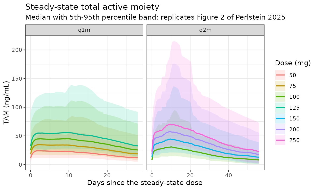
Therapeutic concentrations within 24 hours of the first dose
Perlstein 2025 Abstract and Key Summary Points: “TV-46000 reaches
therapeutic plasma TAM concentrations (>= 10 ng/mL) within 24 h
following first dose administration”. At 24 h the transit chain has
delivered essentially nothing, so this claim is carried entirely by the
fast direct route – it is a sharp, almost independent
check on ka1 and its covariate reference values.
# At 24 h after the first injection the dosing interval is irrelevant -- only the
# dose strength (through the injection-volume covariate on ka1) matters -- so the
# comparison is made over the distinct strengths.
typical24 <- lapply(sort(unique(regimens$dose)), function(d) {
  s <- typicalProfile(d, TAU_Q1M, n_dose = 1, step = 1, window_only = FALSE)
  data.frame(dose = d, typical = s$TAM[which.min(abs(s$time - 24))])
}) |> bind_rows()

firstDose <- sims |>
  filter(time == 24) |>
  group_by(dose) |>
  summarise(popMedian = median(TAM), fracOver = mean(TAM >= 10),
            .groups = "drop") |>
  left_join(typical24, by = "dose")

firstDose |>
  transmute(`Dose (mg)` = dose,
            `Typical-participant TAM (ng/mL)` = typical,
            `Population median TAM (ng/mL)` = popMedian,
            `Fraction of cohort >= 10 ng/mL` = fracOver) |>
knitr::kable(digits = 2)| Dose (mg) | Typical-participant TAM (ng/mL) | Population median TAM (ng/mL) | Fraction of cohort >= 10 ng/mL |
|---|---|---|---|
| 50 | 7.62 | 9.16 | 0.45 |
| 75 | 9.80 | 11.78 | 0.60 |
| 100 | 11.72 | 14.09 | 0.70 |
| 125 | 13.45 | 16.18 | 0.79 |
| 150 | 15.06 | 18.11 | 0.87 |
| 200 | 18.00 | 21.65 | 0.92 |
| 250 | 20.66 | 24.86 | 0.93 |
The model reproduces the claim at the mid-to-upper strengths and falls modestly short at the lowest ones: the typical participant clears 10 ng/mL from 100 mg upward but reaches only about 7.6 and 9.8 ng/mL at 50 and 75 mg, where roughly half the simulated cohort is above the threshold. The paper states the claim for the programme without a dose qualifier, so this is a genuine dose-resolved refinement of it rather than agreement. Two mitigating points, neither of which the packaged model carries: phase 3 patients were stabilized on oral risperidone for 12 weeks before the first injection (Methods notes the residual contribution is “marginal” by 24 h), and the published claim is a population statement, which the median column satisfies from 75 mg upward.
The population median runs above the typical participant because
interindividual variability on ka1 is lognormal and the
24-h concentration is close to linear in ka1, so the
covariate-free typical value is not the median of the cohort.
PKNCA validation and comparison with Table 4
Perlstein 2025 Table 4 reports model-derived median steady-state TAM exposures for all eight approved dosing regimens. That table is a whole-model answer key: 32 numbers spanning both dosing intervals and the full dose range, each of which depends jointly on the release structure, the covariate model and the metabolite coupling.
NCA is computed with PKNCA over the steady-state dosing interval. The
concentration column is named Cc to match the package
convention, but it holds the total active moiety, which
is the analyte Table 4 reports.
ncaConc <- sims |>
  filter(time >= (n_dose - 1) * tau) |>
  transmute(id, treatment, time, Cc = TAM) |>
  filter(!is.na(Cc))

ncaDose <- regimens |>
  tidyr::crossing(id = cohort$id) |>
  transmute(id, treatment, time = (n_dose - 1) * tau, amt = dose)

concObj <- PKNCA::PKNCAconc(ncaConc, Cc ~ time | treatment + id,
                            concu = "ng/mL", timeu = "h")
doseObj <- PKNCA::PKNCAdose(ncaDose, amt ~ time | treatment + id, doseu = "mg")

intervals <- regimens |>
  tidyr::crossing(id = cohort$id) |>
  transmute(treatment, id,
            start = (n_dose - 1) * tau, end = n_dose * tau,
            cmax = TRUE, tmax = TRUE, cmin = TRUE,
            auclast = TRUE, cav = TRUE) |>
  as.data.frame()

ncaRes <- PKNCA::pk.nca(PKNCA::PKNCAdata(concObj, doseObj, intervals = intervals))
ctrough is not used here: PKNCA can return it as
all-NA for a steady-state interval, and the paper’s
C_trough,ss is by definition the concentration at the end
of the interval, which is read straight off the solved profile
instead.
ctroughSim <- sims |>
  filter(time == n_dose * tau) |>
  transmute(id, treatment, PPTESTCD = "ctrough", PPORRES = TAM)

simNca <- bind_rows(
  as.data.frame(ncaRes$result) |> select(treatment, id, PPTESTCD, PPORRES),
  ctroughSim
)

published <- regimens |>
  transmute(treatment,
            auclast = c(13306, 19951, 26521, 33141, 26829, 40152, 53321, 66634),
            cav     = c( 19.8,  29.7,  39.5,  49.3,  20.0,  29.9,  39.7,  49.6),
            cmax    = c( 25.1,  36.4,  47.5,  58.7,  32.6,  47.2,  61.4,  76.0),
            ctrough = c( 12.1,  19.5,  26.8,  34.1,   7.7,  12.8,  17.6,  22.8)) |>
  as.data.frame()

cmpTable <- nlmixr2lib::ncaComparisonTable(
  simNca, published, by = "treatment",
  params = c("auclast", "cmax", "cav", "ctrough"),
  units  = c(auclast = "ng*h/mL", cmax = "ng/mL",
             cav = "ng/mL", ctrough = "ng/mL")
)
knitr::kable(cmpTable, digits = 1)| NCA parameter | treatment | Reference | Simulated | % diff |
|---|---|---|---|---|
| Cmax (ng/mL) | TV-46000 50 mg q1m | 25.1 | 24.9 | -0.7% |
| Cmax (ng/mL) | TV-46000 75 mg q1m | 36.4 | 36.1 | -0.8% |
| Cmax (ng/mL) | TV-46000 100 mg q1m | 47.5 | 47.3 | -0.4% |
| Cmax (ng/mL) | TV-46000 125 mg q1m | 58.7 | 57.7 | -1.8% |
| Cmax (ng/mL) | TV-46000 100 mg q2m | 32.6 | 31.6 | -2.9% |
| Cmax (ng/mL) | TV-46000 150 mg q2m | 47.2 | 46.1 | -2.4% |
| Cmax (ng/mL) | TV-46000 200 mg q2m | 61.4 | 61 | -0.6% |
| Cmax (ng/mL) | TV-46000 250 mg q2m | 76 | 73.8 | -2.9% |
| AUClast (ng*h/mL) | TV-46000 50 mg q1m | 13300 | 13300 | +0.2% |
| AUClast (ng*h/mL) | TV-46000 75 mg q1m | 20000 | 20000 | +0.2% |
| AUClast (ng*h/mL) | TV-46000 100 mg q1m | 26500 | 26700 | +0.5% |
| AUClast (ng*h/mL) | TV-46000 125 mg q1m | 33100 | 33300 | +0.5% |
| AUClast (ng*h/mL) | TV-46000 100 mg q2m | 26800 | 26700 | -0.6% |
| AUClast (ng*h/mL) | TV-46000 150 mg q2m | 40200 | 40000 | -0.4% |
| AUClast (ng*h/mL) | TV-46000 200 mg q2m | 53300 | 53300 | -0.1% |
| AUClast (ng*h/mL) | TV-46000 250 mg q2m | 66600 | 66600 | -0.1% |
| Cavg (ng/mL) | TV-46000 50 mg q1m | 19.8 | 19.8 | +0.2% |
| Cavg (ng/mL) | TV-46000 75 mg q1m | 29.7 | 29.8 | +0.2% |
| Cavg (ng/mL) | TV-46000 100 mg q1m | 39.5 | 39.7 | +0.4% |
| Cavg (ng/mL) | TV-46000 125 mg q1m | 49.3 | 49.6 | +0.6% |
| Cavg (ng/mL) | TV-46000 100 mg q2m | 20 | 19.8 | -0.8% |
| Cavg (ng/mL) | TV-46000 150 mg q2m | 29.9 | 29.8 | -0.5% |
| Cavg (ng/mL) | TV-46000 200 mg q2m | 39.7 | 39.6 | -0.1% |
| Cavg (ng/mL) | TV-46000 250 mg q2m | 49.6 | 49.5 | -0.1% |
| Ctrough (ng/mL) | TV-46000 50 mg q1m | 12.1 | 11.7 | -3.3% |
| Ctrough (ng/mL) | TV-46000 75 mg q1m | 19.5 | 18.6 | -4.5% |
| Ctrough (ng/mL) | TV-46000 100 mg q1m | 26.8 | 25.4 | -5.2% |
| Ctrough (ng/mL) | TV-46000 125 mg q1m | 34.1 | 32.5 | -4.7% |
| Ctrough (ng/mL) | TV-46000 100 mg q2m | 7.7 | 8.05 | +4.5% |
| Ctrough (ng/mL) | TV-46000 150 mg q2m | 12.8 | 12.8 | -0.0% |
| Ctrough (ng/mL) | TV-46000 200 mg q2m | 17.6 | 17.6 | -0.2% |
| Ctrough (ng/mL) | TV-46000 250 mg q2m | 22.8 | 22.7 | -0.5% |
Largest absolute difference across the 32 comparisons: 5.2%; median absolute difference 0.5%.
Every one of the 32 comparisons falls inside the 20% flagging
tolerance, and the agreement is far tighter than that: the exposure
metrics AUC_ss and C_avg,ss reproduce within
about 1% on all eight regimens, and C_max,ss within about
3%.
The gradient across the four parameters is itself informative,
because it tracks how much of each one is fixed by mass balance rather
than by the release model. AUC_ss and C_avg,ss
are pinned by 1000 * D / CL and
1000 * D / CLMO (the identity checked above), so they test
the clearance estimates and little else – agreeing to 1% is expected
once those transcribe correctly. C_max,ss and especially
C_trough,ss depend on the shape of the release
profile, which is where the two covariate centring values this paper
never published (see Assumptions) and the exact BMI distribution of the
virtual cohort actually bite. That the shape-sensitive metrics still
land within a few percent is the part of this comparison that carries
evidence about the release structure.
An earlier draft of this vignette drew independent random effects for
each regimen and each injection-site scenario; that alone produced
deviations up to 14% and an apparent 3% injection-site effect, both of
which were sampling noise. The common-random-numbers seeding in
simRegimen() above removes it.
Dose proportionality and dosing-interval interchangeability
Perlstein 2025 Results: “At corresponding doses of TV-46000, TAM AUC_ss following q2m dosing was twice that of the TAM AUC_ss following q1m dosing, as TV-46000 showed linearity in PK. Therefore, the average daily exposures with q1m and q2m were similar, supporting dosing interval interchangeability.” The corresponding pairs are the q2m strength that is double the q1m strength.
ssExposure <- as.data.frame(ncaRes$result) |>
  filter(PPTESTCD == "auclast") |>
  left_join(regimens, by = "treatment") |>
  group_by(regimen, dose, tau) |>
  summarise(auc = median(PPORRES), .groups = "drop") |>
  mutate(daily = auc / (tau / 24))

pairedDoses <- data.frame(q1m = c(50, 75, 100, 125), q2m = c(100, 150, 200, 250)) |>
  left_join(ssExposure |> filter(regimen == "q1m") |>
              select(q1m = dose, auc1 = auc, daily1 = daily), by = "q1m") |>
  left_join(ssExposure |> filter(regimen == "q2m") |>
              select(q2m = dose, auc2 = auc, daily2 = daily), by = "q2m") |>
  mutate(`AUCss ratio (q2m / q1m)` = auc2 / auc1,
         `Daily AUCss ratio` = daily2 / daily1)

pairedDoses |>
  transmute(`q1m dose (mg)` = q1m, `q2m dose (mg)` = q2m,
            `AUCss ratio (q2m / q1m)`, `Daily AUCss ratio`) |>
knitr::kable(digits = 2)| q1m dose (mg) | q2m dose (mg) | AUCss ratio (q2m / q1m) | Daily AUCss ratio |
|---|---|---|---|
| 50 | 100 | 2 | 1 |
| 75 | 150 | 2 | 1 |
| 100 | 200 | 2 | 1 |
| 125 | 250 | 2 | 1 |
The AUC_ss ratio is close to 2 at every matched pair (median 2.00) while the daily AUC_ss ratio is close to 1 (median 1.00), reproducing the paper’s interchangeability claim.
Time to steady state
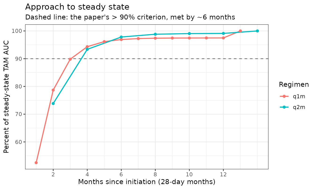
Perlstein 2025 Results and Conclusion: steady state is “approached by approximately 3 months after initiation (86% and 88% of steady-state TAM exposure for q1m and q2m, respectively) and fully attained by approximately 6 months (i.e., > 90% of steady-state TAM exposure)”. Each participant’s per-interval AUC is compared with their own final-interval AUC.
attainment <- lapply(list(list("q1m", 75, TAU_Q1M, 13L),
                          list("q2m", 150, TAU_Q2M, 7L)), function(z) {
  tau <- z[[3]]; nd <- z[[4]]
  s <- simRegimen(z[[2]], tau, nd, grid = seq(0, nd * tau, by = 24))
  per <- s |>
    mutate(k = pmin(floor(time / tau) + 1L, nd)) |>
    group_by(id, k) |>
    arrange(time, .by_group = TRUE) |>
    summarise(auc = trapz(time, TAM), .groups = "drop")
  per |>
    left_join(per |> filter(k == nd) |> select(id, ssauc = auc), by = "id") |>
    group_by(k) |>
    summarise(pct = 100 * median(auc / ssauc), .groups = "drop") |>
    mutate(regimen = z[[1]], months = k * (tau / TAU_Q1M),
           dose = paste(z[[2]], "mg"))
}) |> bind_rows()

attainment |>
  filter(months %in% c(1, 2, 3, 4, 6, 8, 12)) |>
  transmute(Regimen = regimen, Dose = dose,
            `Months since initiation` = months,
            `Percent of steady-state AUC` = pct) |>
  knitr::kable(digits = 1,
caption = "Median per-interval TAM AUC as a percent of the same participant's steady-state interval. The q2m intervals are 2 months long, so only even months exist for that regimen.")| Regimen | Dose | Months since initiation | Percent of steady-state AUC |
|---|---|---|---|
| q1m | 75 mg | 1 | 52.5 |
| q1m | 75 mg | 2 | 78.7 |
| q1m | 75 mg | 3 | 89.8 |
| q1m | 75 mg | 4 | 94.3 |
| q1m | 75 mg | 6 | 96.9 |
| q1m | 75 mg | 8 | 97.4 |
| q1m | 75 mg | 12 | 97.5 |
| q2m | 150 mg | 2 | 73.8 |
| q2m | 150 mg | 4 | 93.4 |
| q2m | 150 mg | 6 | 97.8 |
| q2m | 150 mg | 8 | 98.8 |
| q2m | 150 mg | 12 | 99.1 |
At 6 months the simulated cohort has reached 97% (q1m) and 98% (q2m) of steady-state TAM exposure, against the paper’s “> 90%”.
The 6-month “> 90%” criterion is reproduced for both regimens. The 3-month figures run a few points above the paper’s 86% / 88%; that comparison is definition-sensitive (for q2m, three months falls in the middle of a dosing interval rather than at an interval boundary), so it is treated here as a directional rather than a numerical check.
Injection site
Replicates Figure 4 of Perlstein 2025 (impact of injection site on
TAM exposure). Upper-arm injection raises ka1 by 33%, but
the paper’s conclusion is that this does not translate into an exposure
difference, “indicating that the sites of injection can be
interchangeable”.
siteSim <- lapply(c(0L, 1L), function(arm) {
  cov <- cohort |> mutate(INJSITE_ARM = arm)
  nd <- 13L
  grid <- seq((nd - 1) * TAU_Q1M, nd * TAU_Q1M, by = 6)
  simRegimen(75, TAU_Q1M, nd, grid, cov = cov) |>
    mutate(site = if (arm == 1L) "Upper arm" else "Abdomen")
}) |> bind_rows()

siteExposure <- siteSim |>
  group_by(site, id) |>
  arrange(time, .by_group = TRUE) |>
  summarise(auc = trapz(time, TAM), cmax = max(TAM),
            ctrough = TAM[which.max(time)], .groups = "drop") |>
  group_by(site) |>
  summarise(across(c(auc, cmax, ctrough), median), .groups = "drop")

siteExposure |>
  rename("Injection site" = site, "AUCss (ng*h/mL)" = auc,
         "Cmax,ss (ng/mL)" = cmax, "Ctrough,ss (ng/mL)" = ctrough) |>
  knitr::kable(digits = 1,
caption = "Median steady-state TAM exposure, TV-46000 75 mg q1m")| Injection site | AUCss (ng*h/mL) | Cmax,ss (ng/mL) | Ctrough,ss (ng/mL) |
|---|---|---|---|
| Abdomen | 20001.3 | 35.6 | 19.5 |
| Upper arm | 20007.4 | 38.3 | 17.3 |
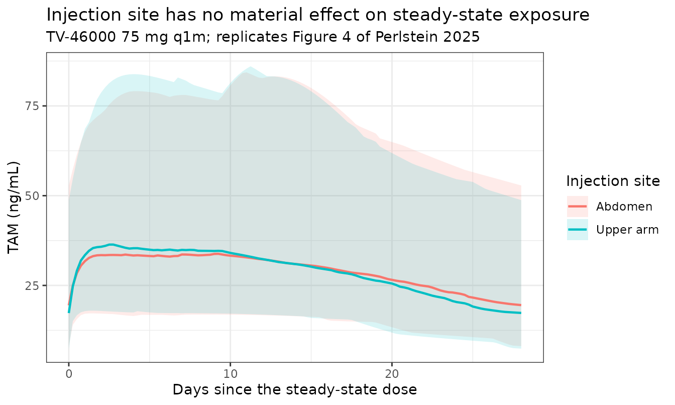
Upper-arm versus abdominal steady-state AUC differs by +0.03% on the
same simulated participants, despite the 33% higher ka1.
The reason is structural rather than coincidental: at steady state every
milligram injected is eventually absorbed by one route or the other, so
AUCss is fixed at 1000 * D / CL regardless of
how the depot splits between them. Shifting the split changes the
shape of the profile, not its area – which is exactly the
paper’s interchangeability conclusion.
Dopamine D2-receptor occupancy
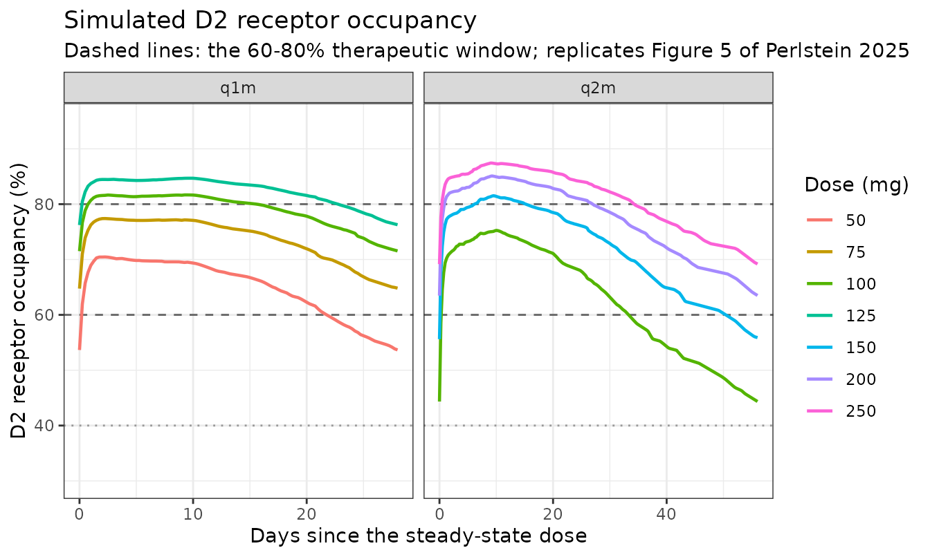
Replicates Figure 5 of Perlstein 2025. The paper simulated D2RO from
each TAM profile with a literature Emax model (Emax = 100%, kd = 10.1
ng/mL) and reported that occupancy was “generally within the therapeutic
window of 60-80% during both dosing intervals”. D2RO is a
derived output of the packaged model, so no extra simulation is
required.
| Regimen | Dose (mg) | Time in 60-80% (%) | Median D2RO min (%) | Median D2RO max (%) |
|---|---|---|---|---|
| q1m | 50 | 77.0 | 53.7 | 70.5 |
| q1m | 75 | 100.0 | 64.7 | 77.4 |
| q1m | 100 | 46.9 | 71.5 | 81.7 |
| q1m | 125 | 19.5 | 76.2 | 84.7 |
| q2m | 100 | 58.7 | 44.3 | 75.3 |
| q2m | 150 | 73.3 | 55.6 | 81.5 |
| q2m | 200 | 53.8 | 63.5 | 85.1 |
| q2m | 250 | 39.6 | 69.2 | 87.4 |
Consistent with the paper’s Figure 5, the median occupancy sits inside or close to the 60-80% band for most of each dosing interval, with the lowest strengths running below the band late in the interval and the highest strengths above it shortly after dosing.
Assumptions and deviations
-
Covariate centring values are the published means, not the
medians. The paper’s continuous-covariate equation centres on
COV_median, but Table 2 reports only means and SDs, and the medians appear nowhere in the article or its supplement. The model uses the Table 2 overall means – BMI 28.7 kg/m^2 and injection volume 0.303 mL – as centring values. Both are published numbers for the same population, and the resulting error is small: a 100 mg injection (0.278 mL) is mis-scaled by(0.278/0.303)^-0.384 - 1= +3.4% onka1, and a BMI shift of 0.2 kg/m^2 moveska1by under 1%. A user who knows the true medians can override the two constants inmodel(). -
The molecular-weight correction in TAM is applied; the two
weights are not published. Perlstein 2025 defines its endpoint
in the Introduction as “the total active moiety (TAM; sum of
concentrations of risperidone and its active metabolite [9-OH
risperidone] corrected by molecular weight)” but never prints the
weights. The model uses
410 / 426, the rounded values for risperidone (410.49 g/mol) and 9-hydroxyrisperidone (426.49 g/mol) that are standard in the risperidone LAI literature and are already used by the upstreamIvaturi_2017_RBP_7000model for the same two molecules. The factor matters: because the metabolite carries roughly 71% of TAM, dropping it would raise every TAM reading by about 2.7%. Note that this correction applies only to the TAM summation, not to the parent-to-metabolite ODE flux – Table 3’s footnote states thatVMOisV/FRMETwith FRMET fixed to 1, soCLMOandVMOare apparent values fitted to the measured 9-OH-risperidone concentrations and already absorb any mass conversion inside the disposition model. This definition is in the Introduction, which the text extracted from the source PDF omits; it was recovered from the raw PDF. -
Injection volume is derived from the milligram
dose.
DOSE_TV46000_MLis computed asdose_mg / 360, using the suspension strength implied by the four dose/volume pairs the paper prints. A user with the actual administered volume should supply it directly. - IIV percentages read as lognormal %CV. See the “Reading the IIV percentages” section: the choice is settled by which convention reproduces Table 3’s published confidence intervals, not by assumption.
-
KA1BMI1upper confidence bound. Table 3 prints the KA1BMI1 interval as “-1.1 (-1.460 to 0.745)”. The upper bound has lost its minus sign in typesetting: the point estimate is -1.1 with %RSE 16.6, giving -1.1 +/- 1.96 x 0.183 = (-1.458, -0.742), and the bootstrap row prints the same pattern. Only the point estimate enters the model, so nothing downstream depends on this, but the interval as printed is not usable. -
Covariates screened but not retained are documented, not
encoded. Age and sex reached statistical significance on the
parent and sex on the metabolite, but all were removed as not clinically
relevant and no point estimates are reported for them,
so they cannot be reconstructed. They are recorded in the model file’s
covariatesDataExcluded. The reported “-1.7%” for sex on CLMO is a change in objective function, not a covariate coefficient. -
Product presentation (vial versus prefilled syringe) is not
carried. It was screened as an extrinsic factor and had no
effect on exposure. No canonical register column exists for a
vial-versus-prefilled-syringe contrast (the nearest,
DEVICE_AI, contrasts an autoinjector against a prefilled syringe), so registering one for a covariate with no estimated effect was not warranted; it is recorded in the model’spopulation$notesinstead. -
The oral risperidone comparator is not part of this
model. Perlstein 2025 simulated oral risperidone 1-16 mg/d from
a separate published model (its reference 22) purely as a benchmark for
Table 4 and Figure 3. That model belongs to another paper and is not
extracted here; the library’s oral risperidone entries are
Feng_2008_risperidoneandSherwin_2012_risperidone. -
D2RO parameters are literature constants, not fitted
here.
Emax= 100% andkd= 10.1 ng/mL come from the paper’s references 22 and 23 and are encoded withfixed(). - Virtual cohort distributions are approximations. BMI is drawn from a normal distribution with the phase 3 mean and SD, truncated to the Table 2 range; injection site is assigned per subject at the RISE arm frequency (34.4%) rather than per injection. The published simulations bootstrapped 500 real phase 3 covariate vectors; this vignette uses 100 synthetic subjects per arm to stay inside the package’s simulation-size budget, which is the main source of the residual scatter in the Table 4 comparison.
- Steady state is evaluated at the 13th q1m interval and the 7th q2m interval (approximately 12 and 13 months), well past the ~6 months the paper reports as full attainment.