Polymyxin B (Wang 2020)
Source:vignettes/articles/Wang_2020_polymyxinB.Rmd
Wang_2020_polymyxinB.RmdModel and source
- Citation: Wang P, Zhang Q, Zhu Z, Feng M, Sun T, Yang J, Zhang X. Population Pharmacokinetics and Limited Sampling Strategy for Therapeutic Drug Monitoring of Polymyxin B in Chinese Patients With Multidrug-Resistant Gram-Negative Bacterial Infections. Front Pharmacol. 2020;11:829. doi:10.3389/fphar.2020.00829. PMCID PMC7289991.
- Description: Two-compartment intravenous population PK model for polymyxin B (sum of polymyxin B1 and B2) in Chinese adults with multidrug-resistant Gram-negative bacterial infections, sampled at steady state on day 4 of therapy (Wang 2020). Cockcroft-Gault creatinine clearance is the sole retained covariate, entering clearance as a power term normalized to 105.9 mL/min with exponent 0.362. Correlated inter-individual variability on V, CL and V2 plus independent variability on Q. Proportional residual error.
- Article: Front Pharmacol. 2020;11:829 (open access, PMC7289991)
Population
Wang 2020 is a single-centre prospective study run at the First Affiliated Hospital of Zhengzhou University (China) between April 2018 and November 2019. Forty-six adults with documented multidrug-resistant Gram-negative bacterial infections, receiving intravenous polymyxin B sulfate for at least 72 hours, contributed 331 plasma concentrations. Patients on renal replacement therapy were excluded. On day 4 of therapy a pre-dose sample (C0h) and five to seven post-dose samples (mainly 0.5, 1, 1.5, 2, 4, 6 and 8 h) were drawn within a single dosing interval. Polymyxin B1 and B2 were measured by LC-MS/MS and summed, so the modelled concentration is total polymyxin B.
The cohort (Table 1) was 39 men and 7 women (15.2% female), median age 46 (range 18-94) years, median weight 70 (45-98) kg, and median Cockcroft-Gault creatinine clearance 89.3 (15.6-315.2) mL/min. Klebsiella pneumoniae (20) and Acinetobacter baumannii (19) were the main pathogens. Daily doses were 100, 150 or 200 mg (median 1.91 mg/kg/day), given q12h mostly as 1-hour infusions (37 patients; 0.5 h in 2, 2 h in 7).
The same information is available programmatically via the model’s
population metadata
(rxode2::rxode(readModelDb("Wang_2020_polymyxinB"))$population).
Source trace
| Model element | Value | Source location |
|---|---|---|
| Two-compartment disposition, IV infusion | – | Results, “Population PK Model”: OFV 1062.13 (one-compartment) vs 694.63 (two-compartment); two-compartment with proportional error chosen as base model |
Exponential IIV, P_i = theta * exp(eta_i)
|
Equ. 1 | Methods, “Population Pharmacokinetics Analysis” |
lvc = log(6.218) |
V 6.218 L | Table 2, row “tvV” (SE 0.83; bootstrap median 5.960, 95% CI 4.169-8.090); Equ. 4 |
lvp = log(11.922) |
V2 11.922 L | Table 2, row “tvV2” (SE 1.74; bootstrap median 12.073); Equ. 5 |
lcl = log(1.786) |
CL 1.786 L/h | Table 2, row “tvCl” (SE 0.12; bootstrap median 1.771); Equ. 6 |
lq = log(13.518) |
Q 13.518 L/h | Table 2, row “tvQ” (SE 3.35; bootstrap median 14.427); Equ. 7 |
e_crcl_cl = 0.362 |
CrCL exponent on CL | Table 2, row “dCldCrCL” (SE 0.09; bootstrap 95% CI 0.196-0.513); exponent of Equ. 6 |
| CrCL normalising constant 105.9 mL/min | – | Equ. 6, Cl = 1.786 x (CrCl/105.9)^0.362 x exp(eta_Cl);
Results text: “105.9 ml/min was the median of CrCL” |
etalvc, etalcl, etalvp
variances |
0.318, 0.208, 0.690 | Table 2, rows “w2 V”, “w2 Cl”, “w2 V2” (footnote: variance of IIV) |
| V-Cl, V-V2, Cl-V2 correlations | 0.713, 0.667, 0.571 | Table 2, rows “CorrV-Cl”, “CorrV-V2”, “CorrCl-V2”; Results text (dOFV = 30.60 for the block) |
etalq variance |
1.508 | Table 2, row “w2 Q” |
propSd |
0.110 | Table 2, row “Residual variability (s) stdev0”; proportional model
Cobs = Cpred x (1 + eps) (Methods) |
The block covariances in ini() are
corr * sqrt(var_i * var_j) from the printed variances and
correlations; the resulting matrix is positive definite.
Virtual cohort and dosing regimens
Table 3 and Figure 3 of the paper simulate three regimens – 100 mg loading then 50 mg q12h, 150 mg loading then 75 mg q12h, and 150 mg loading then 100 mg q12h – infused at 50 mg/h, at three fixed creatinine clearances (31.3, 105.9 and 315.2 mL/min). The loading dose is taken as the first dose at time 0 and the maintenance doses start at 12 h. The paper simulated 1000 patients per scenario; 200 per scenario are used here.
mod <- readModelDb("Wang_2020_polymyxinB")
n_per_arm <- 200L # cap: never more than 200 participants per arm

regimens <- tibble::tribble(
  ~regimen,        ~ld, ~md,
  "50 mg q12h",    100,  50,
  "75 mg q12h",    150,  75,
  "100 mg q12h",   150, 100
)
crcl_levels <- c(31.3, 105.9, 315.2)

arms <- tidyr::expand_grid(regimens, CRCL = crcl_levels) |>
  dplyr::mutate(
    arm = dplyr::row_number(),
    treatment = paste0(regimen, ", CrCL ", CRCL)
  )

subjects <- arms |>
  tidyr::expand_grid(rep = seq_len(n_per_arm)) |>
  dplyr::mutate(id = (arm - 1L) * n_per_arm + rep)

dose_times <- seq(0, 96, by = 12)
doses <- subjects |>
  tidyr::expand_grid(time = dose_times) |>
  dplyr::mutate(
    amt = ifelse(time == 0, ld, md),
    rate = 50, # Methods: 'The infusion rate was set as 50 mg/h'
    evid = 1L,
    cmt = "central"
  )
obs <- subjects |>
  tidyr::expand_grid(time = sort(unique(c(seq(0, 96, by = 0.25))))) |>
  dplyr::mutate(amt = NA_real_, rate = NA_real_, evid = 0L, cmt = "central")

events <- dplyr::bind_rows(doses, obs) |>
  dplyr::select(id, time, amt, rate, evid, cmt, CRCL) |>
  dplyr::arrange(id, time, dplyr::desc(evid)) |>
  as.data.frame()

rxode2::rxSetSeed(20200605)
sim <- rxode2::rxSolve(mod, events, returnType = "data.frame") |>
  dplyr::left_join(
    dplyr::select(subjects, id, arm, regimen, treatment),
    by = "id"
  )
#> ℹ parameter labels from comments will be replaced by 'label()'
arm_key <- dplyr::distinct(arms, arm, regimen, CRCL, treatment)
sim <- sim |>
  dplyr::select(-dplyr::any_of("CRCL")) |>
  dplyr::left_join(dplyr::select(arm_key, arm, CRCL), by = "arm")
Replicate Figure 3: median profiles by CrCL
Replicates Figure 3 of Wang 2020 (median simulated concentration-time profiles for the three regimens in panels by CrCL).
med_prof <- sim |>
  dplyr::group_by(regimen, CRCL, time) |>
  dplyr::summarise(Cc = stats::median(Cc), .groups = "drop") |>
  dplyr::mutate(
    regimen = factor(regimen, levels = regimens$regimen),
    panel = factor(paste0("CrCL ", CRCL, " mL/min"),
                   levels = paste0("CrCL ", crcl_levels, " mL/min"))
  )

ggplot2::ggplot(med_prof, ggplot2::aes(time, Cc, colour = regimen)) +
  ggplot2::geom_line() +
  ggplot2::facet_wrap(~panel) +
  ggplot2::labs(
    x = "Time (h)", y = "Median polymyxin B concentration (mg/L)",
    colour = "Maintenance dose",
    caption = "Replicates Figure 3 of Wang 2020."
  ) +
  ggplot2::theme_bw() +
  ggplot2::theme(legend.position = "bottom")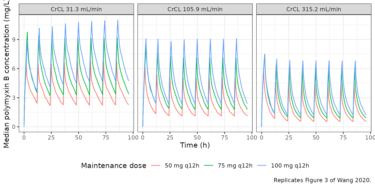
PKNCA validation: day-4 AUC24 and Css,avg (Table 3)
Table 3 reports the day-4 AUC over 24 hours and the average
steady-state concentration. Day 4 is read as 72-96 h after the first
(loading) dose. NCA is run per subject on the individual predictions
Cc (no residual error), grouped by the regimen x CrCL
scenario.
nca_conc <- sim |>
  dplyr::filter(!is.na(Cc), time >= 72, time <= 96) |>
  dplyr::select(id, time, Cc, treatment)
nca_dose <- doses |>
  dplyr::filter(time >= 72, time < 96) |>
  dplyr::select(id, time, amt, treatment)

conc_obj <- PKNCA::PKNCAconc(nca_conc, Cc ~ time | treatment + id,
                             concu = "mg/L", timeu = "h")
dose_obj <- PKNCA::PKNCAdose(nca_dose, amt ~ time | treatment + id,
                             doseu = "mg")
intervals <- data.frame(start = 72, end = 96, auclast = TRUE, cav = TRUE,
                        cmax = TRUE, cmin = TRUE)
nca_res <- PKNCA::pk.nca(PKNCA::PKNCAdata(conc_obj, dose_obj,
                                          intervals = intervals))
nca_long <- as.data.frame(nca_res) |>
  dplyr::select(treatment, id, PPTESTCD, PPORRES)
The reference values are the Table 3 medians (P50);
ncaComparisonTable() also aggregates the simulated subjects
by the median, so the two sides are the same statistic.
table3 <- tibble::tribble(
  ~regimen,      ~CRCL, ~auc_p5, ~auc_p50, ~auc_p95, ~cav_p5, ~cav_p50, ~cav_p95,
  "50 mg q12h",   31.3,  36.93,   87.20,  192.19,   1.54,   3.63,   8.01,
  "50 mg q12h",  105.9,  23.85,   53.33,  118.77,   0.99,   2.22,   4.95,
  "50 mg q12h",  315.2,  15.54,   37.92,   84.49,   0.65,   1.58,   3.52,
  "75 mg q12h",   31.3,  56.60,  128.58,  295.12,   2.36,   5.36,  12.30,
  "75 mg q12h",  105.9,  35.15,   82.04,  180.81,   1.46,   3.42,   7.53,
  "75 mg q12h",  315.2,  22.46,   53.60,  121.32,   0.94,   2.23,   5.06,
  "100 mg q12h",  31.3,  75.39,  167.90,  364.58,   3.14,   7.00,  15.19,
  "100 mg q12h", 105.9,  49.23,  108.57,  247.01,   2.05,   4.52,  10.29,
  "100 mg q12h", 315.2,  30.29,   71.91,  167.40,   1.26,   3.00,   6.98
) |>
  dplyr::mutate(treatment = paste0(regimen, ", CrCL ", CRCL))

reference <- table3 |>
  dplyr::transmute(treatment, auclast = auc_p50, cav = cav_p50)

cmp <- nlmixr2lib::ncaComparisonTable(
  simulated = nca_long,
  reference = reference,
  by = "treatment",
  params = c("auclast", "cav"),
  units = c(auclast = "mg*h/L", cav = "mg/L"),
  tolerance_pct = 20
)
cmp |>
  dplyr::rename("Scenario" = treatment) |>
  knitr::kable(caption = paste(
    "Simulated day-4 (72-96 h) AUC and average concentration versus the",
    "Wang 2020 Table 3 medians. AUC0-24 on day 4 is reported by PKNCA as",
    "AUClast over the 72-96 h interval."
))| NCA parameter | Scenario | Reference | Simulated | % diff |
|---|---|---|---|---|
| AUClast (mg*h/L) | 50 mg q12h, CrCL 31.3 | 87.2 | 87.9 | +0.8% |
| AUClast (mg*h/L) | 50 mg q12h, CrCL 105.9 | 53.3 | 51.9 | -2.7% |
| AUClast (mg*h/L) | 50 mg q12h, CrCL 315.2 | 37.9 | 37.1 | -2.2% |
| AUClast (mg*h/L) | 75 mg q12h, CrCL 31.3 | 129 | 129 | +0.3% |
| AUClast (mg*h/L) | 75 mg q12h, CrCL 105.9 | 82 | 84.9 | +3.5% |
| AUClast (mg*h/L) | 75 mg q12h, CrCL 315.2 | 53.6 | 56.3 | +5.0% |
| AUClast (mg*h/L) | 100 mg q12h, CrCL 31.3 | 168 | 172 | +2.3% |
| AUClast (mg*h/L) | 100 mg q12h, CrCL 105.9 | 109 | 112 | +3.1% |
| AUClast (mg*h/L) | 100 mg q12h, CrCL 315.2 | 71.9 | 74.3 | +3.3% |
| Cavg (mg/L) | 50 mg q12h, CrCL 31.3 | 3.63 | 3.66 | +0.9% |
| Cavg (mg/L) | 50 mg q12h, CrCL 105.9 | 2.22 | 2.16 | -2.6% |
| Cavg (mg/L) | 50 mg q12h, CrCL 315.2 | 1.58 | 1.54 | -2.2% |
| Cavg (mg/L) | 75 mg q12h, CrCL 31.3 | 5.36 | 5.37 | +0.3% |
| Cavg (mg/L) | 75 mg q12h, CrCL 105.9 | 3.42 | 3.54 | +3.4% |
| Cavg (mg/L) | 75 mg q12h, CrCL 315.2 | 2.23 | 2.34 | +5.1% |
| Cavg (mg/L) | 100 mg q12h, CrCL 31.3 | 7 | 7.16 | +2.3% |
| Cavg (mg/L) | 100 mg q12h, CrCL 105.9 | 4.52 | 4.66 | +3.2% |
| Cavg (mg/L) | 100 mg q12h, CrCL 315.2 | 3 | 3.09 | +3.1% |
The simulated medians reproduce the Table 3 medians to within a few percent in every scenario, including the covariate direction (lower CrCL, higher exposure) and its magnitude across the 10-fold CrCL range.
The 5th and 95th percentiles of Table 3 are compared as well. These are tail quantiles of a 200-subject cohort, so they are shown for context and are not asserted on.
sim_q <- nca_long |>
  dplyr::filter(PPTESTCD == "auclast") |>
  dplyr::group_by(treatment) |>
  dplyr::summarise(
    sim_p5 = stats::quantile(PPORRES, 0.05),
    sim_p50 = stats::median(PPORRES),
    sim_p95 = stats::quantile(PPORRES, 0.95),
    .groups = "drop"
  ) |>
  dplyr::inner_join(table3, by = "treatment") |>
  dplyr::mutate(pct_diff_p50 = 100 * (sim_p50 - auc_p50) / auc_p50) |>
  dplyr::arrange(match(treatment, table3$treatment))

sim_q |>
  dplyr::select(treatment, auc_p5, sim_p5, auc_p50, sim_p50, auc_p95,
                sim_p95, pct_diff_p50) |>
  dplyr::rename(
    "Scenario" = treatment,
    "P5 paper" = auc_p5, "P5 sim" = sim_p5,
    "P50 paper" = auc_p50, "P50 sim" = sim_p50,
    "P95 paper" = auc_p95, "P95 sim" = sim_p95,
    "P50 % diff" = pct_diff_p50
  ) |>
  knitr::kable(digits = 1, caption = paste(
    "Day-4 AUC24 (mg*h/L) percentiles: Wang 2020 Table 3 versus simulation."
))| Scenario | P5 paper | P5 sim | P50 paper | P50 sim | P95 paper | P95 sim | P50 % diff |
|---|---|---|---|---|---|---|---|
| 50 mg q12h, CrCL 31.3 | 36.9 | 40.7 | 87.2 | 87.9 | 192.2 | 185.8 | 0.8 |
| 50 mg q12h, CrCL 105.9 | 23.9 | 25.5 | 53.3 | 51.9 | 118.8 | 105.8 | -2.7 |
| 50 mg q12h, CrCL 315.2 | 15.5 | 16.8 | 37.9 | 37.1 | 84.5 | 85.7 | -2.2 |
| 75 mg q12h, CrCL 31.3 | 56.6 | 62.4 | 128.6 | 129.0 | 295.1 | 286.8 | 0.3 |
| 75 mg q12h, CrCL 105.9 | 35.1 | 38.4 | 82.0 | 84.9 | 180.8 | 176.6 | 3.5 |
| 75 mg q12h, CrCL 315.2 | 22.5 | 27.8 | 53.6 | 56.3 | 121.3 | 130.0 | 5.0 |
| 100 mg q12h, CrCL 31.3 | 75.4 | 79.8 | 167.9 | 171.8 | 364.6 | 345.0 | 2.3 |
| 100 mg q12h, CrCL 105.9 | 49.2 | 52.7 | 108.6 | 111.9 | 247.0 | 214.1 | 3.1 |
| 100 mg q12h, CrCL 315.2 | 30.3 | 37.9 | 71.9 | 74.3 | 167.4 | 156.9 | 3.3 |
stopifnot(
  # Structural: a mis-transcribed clearance, exponent or normalising constant
  # moves every scenario by tens of percent.
  abs(stats::median(sim_q$pct_diff_p50)) < 5,
  # Envelope across the nine scenarios, robust to the sampling noise of a
  # 200-subject median (about 4% for the ~46% CV on CL).
  stats::quantile(abs(sim_q$pct_diff_p50), 0.9) < 12
)
Typical-value closed-form check
For a linear two-compartment model at true steady state, the AUC over
one 24-hour window equals the dose given in that window divided by CL,
independently of the distribution parameters. With random effects zeroed
and dosing continued for 20 days (the typical terminal half-life is well
under one day), the integrated AUC must reproduce
2 x MD / CL at every CrCL. This exercises the covariate
term and the ODE wiring without any random draw, so a tight bound is
appropriate.
mod_tv <- rxode2::zeroRe(mod)
#> ℹ parameter labels from comments will be replaced by 'label()'
tv_subj <- tibble::tibble(id = seq_along(crcl_levels), CRCL = crcl_levels)
tv_events <- dplyr::bind_rows(
  tv_subj |>
    tidyr::expand_grid(time = seq(0, 480 + 12, by = 12)) |>
    dplyr::mutate(amt = 50, rate = 50, evid = 1L, cmt = "central"),
  tv_subj |>
    tidyr::expand_grid(time = seq(480, 504, by = 0.05)) |>
    dplyr::mutate(amt = NA_real_, rate = NA_real_, evid = 0L,
                  cmt = "central")
) |>
  dplyr::arrange(id, time, dplyr::desc(evid)) |>
  as.data.frame()

tv_sim <- rxode2::rxSolve(mod_tv, tv_events, returnType = "data.frame")
#> ℹ omega/sigma items treated as zero: 'etalvc', 'etalcl', 'etalvp', 'etalq'
#> Warning: multi-subject simulation without without 'omega'
tv_check <- tv_sim |>
  dplyr::group_by(id) |>
  dplyr::summarise(
    CRCL = dplyr::first(CRCL),
    cl = dplyr::first(cl),
    auc = sum(diff(time) * (utils::head(Cc, -1) + utils::tail(Cc, -1)) / 2),
    .groups = "drop"
  ) |>
  dplyr::mutate(
    cl_expected = 1.786 * (CRCL / 105.9)^0.362,
    auc_expected = 2 * 50 / cl_expected,
    pct_diff = 100 * (auc - auc_expected) / auc_expected
  )

tv_check |>
  dplyr::select(CRCL, cl, cl_expected, auc, auc_expected, pct_diff) |>
  dplyr::rename(
    "CrCL (mL/min)" = CRCL, "CL model (L/h)" = cl,
    "CL Equ. 6 (L/h)" = cl_expected, "AUC24 integrated" = auc,
    "2 x 50 mg / CL" = auc_expected, "% diff" = pct_diff
  ) |>
knitr::kable(digits = 4, caption = "Typical-value steady-state AUC24 at 50 mg q12h.")| CrCL (mL/min) | CL model (L/h) | CL Equ. 6 (L/h) | AUC24 integrated | 2 x 50 mg / CL | % diff |
|---|---|---|---|---|---|
| 31.3 | 1.1488 | 1.1488 | 87.0450 | 87.0450 | 0 |
| 105.9 | 1.7860 | 1.7860 | 55.9910 | 55.9910 | 0 |
| 315.2 | 2.6507 | 2.6507 | 37.7262 | 37.7262 | 0 |
Observed-cohort AUC0-12
The paper reports an observed (non-compartmental) AUC0-12h of 43.64 +/- 27.68 mg*h/L (range 8.50-122.84) across the 46 patients. A rough virtual version of that cohort is simulated below: maintenance doses of 50, 75 or 100 mg q12h in the Table 1 proportions (25 : 15 : 8 patients), 1-hour infusions, and a creatinine clearance drawn log-normally around the Table 1 median of 89.3 mL/min and truncated to the observed 15.6-315.2 mL/min range. Dosing runs for 4 days without a loading dose (the cohort loading practice is not reported per patient) and the day-4 interval 72-84 h is analysed. This is descriptive only – the paper does not report the covariate distribution in enough detail for a sharp comparison.
n_cohort <- 200L
rxode2::rxSetSeed(46)
cohort <- tibble::tibble(
  id = seq_len(n_cohort),
  md = sample(c(50, 75, 100), n_cohort, replace = TRUE,
              prob = c(25, 15, 8)),
  CRCL = pmin(pmax(exp(stats::rnorm(n_cohort, log(89.3), 0.75)), 15.6), 315.2)
)
coh_events <- dplyr::bind_rows(
  cohort |>
    tidyr::expand_grid(time = seq(0, 84, by = 12)) |>
    dplyr::mutate(amt = md, rate = md, evid = 1L, cmt = "central"),
  cohort |>
    tidyr::expand_grid(time = seq(72, 84, by = 0.1)) |>
    dplyr::mutate(amt = NA_real_, rate = NA_real_, evid = 0L,
                  cmt = "central")
) |>
  dplyr::select(id, time, amt, rate, evid, cmt, CRCL) |>
  dplyr::arrange(id, time, dplyr::desc(evid)) |>
  as.data.frame()
coh_sim <- rxode2::rxSolve(mod, coh_events, returnType = "data.frame")
coh_auc <- coh_sim |>
  dplyr::filter(!is.na(Cc)) |>
  dplyr::group_by(id) |>
  dplyr::summarise(
    auc = sum(diff(time) * (utils::head(Cc, -1) + utils::tail(Cc, -1)) / 2),
    .groups = "drop"
  )
tibble::tibble(
  Source = c("Wang 2020 observed (n = 46)", "Simulated virtual cohort"),
  `Mean AUC0-12 (mg*h/L)` = c(43.64, mean(coh_auc$auc)),
  `SD` = c(27.68, stats::sd(coh_auc$auc)),
  `Min` = c(8.50, min(coh_auc$auc)),
  `Max` = c(122.84, max(coh_auc$auc))
) |>
knitr::kable(digits = 2, caption = "Day-4 AUC0-12: observed versus a virtual cohort.")| Source | Mean AUC0-12 (mg*h/L) | SD | Min | Max |
|---|---|---|---|---|
| Wang 2020 observed (n = 46) | 43.64 | 27.68 | 8.50 | 122.84 |
| Simulated virtual cohort | 44.16 | 26.91 | 9.86 | 179.49 |
Assumptions and deviations
- CrCL normalising constant. Equ. 6 normalises CrCL by 105.9 mL/min and the Results text calls 105.9 “the median of CrCL”, whereas Table 1 reports the cohort CrCL as median 89.3 (range 15.6-315.2) mL/min. The Methods also use 105.9 as the “medium” value of the Table 3 simulations. The printed equation is followed (105.9). The typical clearance at the Table 1 median of 89.3 mL/min is then 1.68 L/h rather than 1.786 L/h. The source of the discrepancy (e.g. median over samples rather than patients, or over a subset) is not stated.
-
Covariate units. CrCL is the raw Cockcroft-Gault
estimate in mL/min (not normalised to 1.73 m^2) and is stored in the
canonical
CRCLcolumn with mL/min units, as in other raw Cockcroft-Gault models in the library. - Dose units. The Methods quote the Chinese label as “50 to 100 million units (1 million units equal to 1 mg) twice daily”; the conventional polymyxin B conversion is 10,000 units per mg, so the stated unit numbers appear to be a translation slip. All doses in the paper’s tables and simulations are in mg, and the model is dosed in mg.
- Table 1 dose counts. The daily-dose counts (25 + 15 + 8 = 48) exceed the 46 patients and “25 (50.0%)” does not match 25/46; the proportions are used only for the descriptive virtual cohort.
- Day-4 window for Table 3. “AUC24h … on day four” is read as 72-96 h after the loading dose, with maintenance doses starting at 12 h. The paper does not state the dosing clock explicitly.
- Parameter classification. The Table 2 footnote calls dCldCrCL a “fixed parameter coefficient”; in Phoenix NLME terminology this denotes a fixed effect (theta), and the parameter has an SE and bootstrap CI, so it is encoded as estimated.
- Limited sampling strategies. The Bayesian and multiple-linear-regression limited sampling equations for AUC0-12h (Tables 4-5) are TDM estimation tools derived from the observed data, not part of the population model, and are not encoded.
- No errata were found for this article (literature check, September 2026). The supplement (Supplementary Figure 1, CrCL versus individual CL) contains no parameter values.