Brepocitinib (Hughes 2022) • nlmixr2lib

Model and source

Citation: Hughes JH, Qiu R, Banfield C, Dowty ME, Nicholas T. Population pharmacokinetics of oral brepocitinib in healthy volunteers and patients. Clinical Pharmacology in Drug Development. 2022;11(12):1447-1456. doi:10.1002/cpdd.1163
Description: One-compartment population pharmacokinetic model with first-order absorption and a tablet-only absorption lag for oral brepocitinib (PF-06700841, a dual TYK2/JAK1 inhibitor) in healthy participants and patients with plaque psoriasis or alopecia areata. Apparent clearance and apparent central volume carry allometric body-weight scaling with exponents fixed to literature values at a 70 kg reference, and apparent clearance is 24.3 percent lower in Asian participants. A high-fat meal slows absorption by 69.9 percent and lowers relative bioavailability by 28.3 percent, while doses of 175 mg and above raise relative bioavailability by 35.1 percent. Interindividual variability on CL/F and Vc/F is correlated, and the log-scale residual error differs between the phase 1 healthy-volunteer studies and the phase 2 patient studies.
Article: https://doi.org/10.1002/cpdd.1163

Brepocitinib (PF-06700841) is an oral tyrosine kinase 2 (TYK2) and Janus kinase 1 (JAK1) inhibitor. Hughes 2022 is the first published population pharmacokinetic analysis of the programme. A later and larger analysis of the same molecule, pooling nine studies and 775 subjects into a two-compartment model, is packaged separately as Maleki_2024_brepocitinib.

Population

The analysis pooled 5541 plasma brepocitinib observations from 379 subjects in five trials: three phase 1 studies in healthy participants (NCT02310750, the first-in-human single- and multiple-ascending-dose and food-effect study; NCT03236493, a multiple-dose study in healthy Japanese participants; and NCT03656952, a concentration-QT study) and two phase 2 patient studies (NCT02969018 in moderate-to-severe plaque psoriasis and NCT02974868 in moderate-to-severe alopecia areata).

Baseline demographics (Hughes 2022 Table 2): median age 42 years (range 18-75), median body weight 83 kg (range 45-204), median creatinine clearance 124 mL/min (range 58-279). 69% of subjects were male. Race was 82% White, 8% Asian, 5% African American and 6% Other. 24% were healthy participants, 55% had plaque psoriasis and 20% had alopecia areata. 83% received tablets and 17% the oral suspension used in the first-in-human study.

Doses spanned 1-200 mg. The phase 1 studies contributed single doses of 1, 3, 10, 30, 100 and 200 mg and multiple doses of 10, 30, 100 and 175 mg once daily or 50 mg twice daily; the phase 2 studies contributed 30 or 60 mg once-daily induction followed by 10 or 30 mg once-daily maintenance. 10.8% of observations were missing or below the 0.2 ng/mL limit of quantification and were treated as missing; an M3 sensitivity analysis moved only the CL/F interindividual variability.

The same information is available programmatically via readModelDb("Hughes_2022_brepocitinib")()$population.

Source trace

Every ini() entry in inst/modeldb/specificDrugs/Hughes_2022_brepocitinib.R carries an in-file comment naming its origin. They are collected here for review.

Equation / parameter	Value	Source location
`lka` (ka)	3.46 1/h (95% CI 3.04-3.88)	Table 3, “First-order absorption rate constant”; Equation 7
`lcl` (CL/Frel)	18.7 L/h (16.9-20.5)	Table 3, “Apparent clearance (CL/F)”; Equation 9
`lvc` (Vc/Frel)	136 L (124-148)	Table 3, “Apparent volume of distribution (Vc/F)”; Equation 10
`ltlag` (Alag)	0.240 h (0.234-0.246)	Table 3, “Absorption lag”; Equation 6
`lfdepot` (Frel)	1 (structural anchor, fixed)	Equation 8, the leading `1 *`; no Table 3 row
`e_wt_cl`	0.750 (fixed)	Table 3, “Effect of weight on CL/F (70 kg reference)”; Equation 9
`e_wt_vc`	1.00 (fixed)	Table 3, “Effect of weight on Vc/F (70 kg reference)”; Equation 10
`e_form_suspension_tlag`	-1.00 (fixed)	Table 3, “Effect of suspension formulation on Alag”; Equation 6
`e_fed_highfat_ka`	-0.699 (-0.899 to -0.499)	Table 3, “Effect of high-fat meal on ka”; Equation 7
`e_race_asian_cl`	-0.243 (-0.363 to -0.123)	Table 3, “Effect of Asian subjects on CL/F”; Equation 9
`e_fed_highfat_fdepot`	-0.283 (-0.389 to -0.177)	Table 3, “Effect of high-fat meal on Frel”; Equation 8
`e_dose_high_fdepot`	0.351 (0.194 to 0.508)	Table 3, “Effect of dose on Frel (dose >= 175 mg)”; Equation 8
`var(etalcl)`	0.6084 = 0.780^2	Table 3, “omega CL/F (% CV)” = 78.0 (57.5-98.5)
`var(etalvc)`	0.366025 = 0.605^2	Table 3, “omega Vc/F (%CV)” = 60.5 (27.3-93.5)
`cov(etalcl, etalvc)`	0.358644 = 0.760 x 0.780 x 0.605	Table 3, “rho CL/F-Vc/F” = 0.760 (0.403-1.12)
`expSdHv`	0.527 (0.444-0.610)	Table 3, “Proportional RUV (phase 1;CV)”; Equation 2
`expSdPat`	0.875 (0.812-0.938)	Table 3, “Proportional RUV (phase 2;CV)”; Equation 2
Categorical covariate form `P * (1 + theta * COV)`	n/a	Equation 4
Continuous covariate form `P * (COV/COVref)^theta`	n/a	Equation 5
One-compartment ODE with first-order absorption	n/a	Base Model and Discussion; Equations 6-10
Log-transform-both-sides proportional residual error	n/a	Equation 2

Reading the reported “% CV”

The interindividual-variability rows of Table 3 are labelled omega CL/F (% CV) and omega Vc/F (%CV), so the tabulated quantity is omega itself expressed as a percentage, not the log-normal coefficient of variation sqrt(exp(omega^2) - 1). Two independent confirmations sit in the same table. First, the residual-error rows use the identical CV label for a quantity Equation 2 defines unambiguously as a log-scale standard deviation: ln(DV) = ln(IPRED) + theta_pro * eps with Var(eps) fixed at 1, and Table 3 reports theta_pro = 0.527. Second, the reported 95% confidence intervals are exactly symmetric about the point estimates on this scale (78.0 with 57.5 to 98.5; 60.5 with 27.3 to 93.5), as an SD-scale interval would be. The model file therefore uses omega_CL/F = 0.780 and omega_Vc/F = 0.605. For reference, the equivalent true log-normal CVs are 91.5% and 66.3%.

Deterministic covariate checks

The paper’s quantitative claims are all statements about typical values, so they are checked here on random-effect-free (zeroRe) solves where each ratio is an exact identity of the published equations rather than a draw from a simulated cohort.

mod <- readModelDb("Hughes_2022_brepocitinib")
mod_typ <- rxode2::zeroRe(mod)
#> Warning: No sigma parameters in the model

# Observation grid: 0.01 h out to 6 h so that Tmax (and the 0.240 h absorption
# lag) resolve cleanly, then 0.1 h out to 48 h -- about 9.5 elimination
# half-lives -- so that lambda-z and the AUC extrapolation are well determined.
obs_times <- sort(unique(c(seq(0, 6, by = 0.01), seq(6, 48, by = 0.1))))

# One scenario = one subject. Doses go to the named ODE state `depot` and
# observations to the named ODE state `central`; rxode2 returns the algebraic
# observable Cc alongside, so an algebraic observable must never be named as a
# compartment here -- doing so injects a slot and renumbers the ODE states.
make_scenario <- function(id, scenario, dose, wt = 70, asian = 0, fed = 0,
                          tablet = 1, dose_high = 0, healthy = 1,
                          n_doses = 1L, tau = 24, times = obs_times) {
  dose_times <- (seq_len(n_doses) - 1L) * tau
  ev <- dplyr::bind_rows(
    data.frame(time = dose_times, amt = dose, evid = 1L, cmt = "depot"),
    data.frame(time = max(dose_times) + times, amt = NA_real_,
               evid = 0L, cmt = "central")
  )
  ev$id <- id
  ev$scenario <- scenario
  ev$WT <- wt
  ev$RACE_ASIAN <- asian
  ev$FED_HIGHFAT <- fed
  ev$FORM_TABLET <- tablet
  ev$DOSE_HIGH <- dose_high
  ev$DIS_HEALTHY <- healthy
  ev[order(ev$time, -ev$evid), ]
}

# Reference individual per Hughes 2022 Figure 1: 70 kg, non-Asian, tablet,
# dosed below 175 mg and without regard to food.
ev_typ <- dplyr::bind_rows(
  make_scenario(1L, "30 mg tablet",              dose = 30),
  make_scenario(2L, "30 mg tablet, Asian",       dose = 30, asian = 1),
  make_scenario(3L, "30 mg tablet, high-fat",    dose = 30, fed = 1),
  make_scenario(4L, "30 mg suspension",          dose = 30, tablet = 0),
  make_scenario(5L, "30 mg tablet, 100 kg",      dose = 30, wt = 100),
  make_scenario(6L, "200 mg tablet",             dose = 200, dose_high = 1),
  make_scenario(7L, "200 mg tablet, linear",     dose = 200, dose_high = 0)
)

sim_typ <- rxode2::rxSolve(
  mod_typ, events = ev_typ, keep = "scenario", omega = NA, returnType = "data.frame"
)
#> Warning: multi-subject simulation without without 'omega'
str(sim_typ[, c("id", "time", "Cc", "scenario")])
#> 'data.frame':    7147 obs. of  4 variables:
#>  $ id      : int  1 1 1 1 1 1 1 1 1 1 ...
#>  $ time    : num  0 0.01 0.02 0.03 0.04 0.05 0.06 0.07 0.08 0.09 ...
#>  $ Cc      : num  0 0 0 0 0 0 0 0 0 0 ...
#>  $ scenario: chr  "30 mg tablet" "30 mg tablet" "30 mg tablet" "30 mg tablet" ...

sim_nca <- sim_typ |>
  dplyr::filter(!is.na(Cc)) |>
  dplyr::select(id, time, Cc, scenario)

# Guarantee a time-zero row per subject; brepocitinib is given orally, so a
# pre-dose concentration of 0 is the correct anchor for AUC0-*.
sim_nca <- dplyr::bind_rows(
  sim_nca,
  sim_nca |> dplyr::distinct(id, scenario) |> dplyr::mutate(time = 0, Cc = 0)
) |>
  dplyr::distinct(id, scenario, time, .keep_all = TRUE) |>
  dplyr::arrange(id, scenario, time)

dose_df <- ev_typ |>
  dplyr::filter(evid == 1) |>
  dplyr::select(id, time, amt, scenario)

conc_obj <- PKNCA::PKNCAconc(sim_nca, Cc ~ time | scenario + id,
                             concu = "ng/mL", timeu = "h")
dose_obj <- PKNCA::PKNCAdose(dose_df, amt ~ time | scenario + id, doseu = "mg")

intervals_sd <- data.frame(
  start = 0, end = Inf,
  cmax = TRUE, tmax = TRUE, aucinf.obs = TRUE, half.life = TRUE
)

nca_typ <- PKNCA::pk.nca(
  PKNCA::PKNCAdata(conc_obj, dose_obj, intervals = intervals_sd)
)

nca_wide <- as.data.frame(nca_typ) |>
  dplyr::select(scenario, PPTESTCD, PPORRES) |>
  tidyr::pivot_wider(names_from = PPTESTCD, values_from = PPORRES)

get_val <- function(scen, param) {
  nca_wide[[param]][match(scen, nca_wide$scenario)]
}

knitr::kable(
  nca_wide |>
    dplyr::rename(
      "Scenario"          = scenario,
      "Cmax (ng/mL)"      = cmax,
      "Tmax (h)"          = tmax,
      "AUC0-inf (ng*h/mL)" = aucinf.obs,
      "t1/2 (h)"          = half.life
    ),
  digits = 3,
  caption = "Typical-value (zero random effect) NCA for each covariate scenario."
)

Typical-value (zero random effect) NCA for each covariate scenario.
Scenario	Cmax (ng/mL)	Tmax (h)	tlast	clast.obs	lambda.z	r.squared	adj.r.squared	lambda.z.time.first	lambda.z.time.last	lambda.z.n.points	clast.pred	t1/2 (h)	span.ratio	AUC0-inf (ng*h/mL)
200 mg tablet	1738.506	1.21	48	2.909	0.137	1	1	1.22	48	899	2.913	5.044	9.274	14449.152
200 mg tablet, linear	1286.829	1.21	48	2.153	0.137	1	1	1.22	48	899	2.156	5.044	9.274	10695.153
30 mg suspension	193.024	0.97	48	0.312	0.137	1	1	0.98	48	923	0.313	5.044	9.322	1604.273
30 mg tablet	193.024	1.21	48	0.323	0.137	1	1	1.22	48	899	0.323	5.044	9.274	1604.273
30 mg tablet, 100 kg	136.264	1.23	48	0.395	0.126	1	1	1.24	48	897	0.395	5.515	8.479	1227.728
30 mg tablet, Asian	197.872	1.28	48	1.577	0.104	1	1	1.29	48	892	1.579	6.663	7.010	2119.260
30 mg tablet, high-fat	116.238	2.48	48	0.256	0.137	1	1	2.81	48	740	0.260	5.075	8.904	1150.278

The NCA instrument agrees with the closed form

Before the published claims are checked, the NCA itself is checked against the analytic solution of the model, so that a discrepancy below can be attributed to the transcription rather than to the measurement.

cl_ref  <- 18.7                      # L/h, Table 3
vc_ref  <- 136                       # L,   Table 3
ka_ref  <- 3.46                      # 1/h, Table 3
tlag    <- 0.240                     # h,   Table 3
kel_ref <- cl_ref / vc_ref

# For a one-compartment model with complete first-order absorption,
# AUC0-inf = Dose * Frel / CL, exactly, independent of ka and of the lag.
auc_closed_form <- 30 * 1 / cl_ref * 1000       # mg/(L/h) -> ng*h/mL
hl_closed_form  <- log(2) * vc_ref / cl_ref
tmax_closed_tab <- log(ka_ref / kel_ref) / (ka_ref - kel_ref) + tlag

instrument <- tibble::tibble(
  Quantity = c("AUC0-inf, 30 mg tablet (ng*h/mL)", "t1/2 (h)", "Tmax, tablet (h)"),
  `Closed form` = c(auc_closed_form, hl_closed_form, tmax_closed_tab),
  PKNCA = c(get_val("30 mg tablet", "aucinf.obs"),
            get_val("30 mg tablet", "half.life"),
            get_val("30 mg tablet", "tmax"))
) |>
  dplyr::mutate(`% diff` = (PKNCA - `Closed form`) / `Closed form` * 100)

knitr::kable(instrument, digits = 4,
             caption = "PKNCA against the analytic solution of the same model.")

PKNCA against the analytic solution of the same model.
Quantity	Closed form	PKNCA	% diff
AUC0-inf, 30 mg tablet (ng*h/mL)	1604.2781	1604.2729	-0.0003
t1/2 (h)	5.0411	5.0441	0.0609
Tmax, tablet (h)	1.2108	1.2100	-0.0640


# The solve is deterministic, so these are numerical-integration differences
# only: no cohort is drawn and nothing here varies with the solver thread count.
# Tmax is resolved only to the 0.01 h observation grid, hence its own bound.
stopifnot(
  abs(instrument$`% diff`[instrument$Quantity != "Tmax, tablet (h)"]) < 1,
  abs(get_val("30 mg tablet", "tmax") - tmax_closed_tab) < 0.02
)

Published covariate claims

auc_ref     <- get_val("30 mg tablet", "aucinf.obs")
auc_asian   <- get_val("30 mg tablet, Asian", "aucinf.obs")
auc_fed     <- get_val("30 mg tablet, high-fat", "aucinf.obs")
auc_wt100   <- get_val("30 mg tablet, 100 kg", "aucinf.obs")
auc_200_hi  <- get_val("200 mg tablet", "aucinf.obs")
auc_200_lin <- get_val("200 mg tablet, linear", "aucinf.obs")

tmax_tab  <- get_val("30 mg tablet", "tmax")
tmax_susp <- get_val("30 mg suspension", "tmax")
tmax_fed  <- get_val("30 mg tablet, high-fat", "tmax")

# ka is not an NCA parameter, so the high-fat absorption-rate claim is checked
# through the Tmax it implies, computed in closed form from the model's own ka.
ka_fed          <- ka_ref * (1 - 0.699)
tmax_closed_fed <- log(ka_fed / kel_ref) / (ka_fed - kel_ref) + tlag

claims <- tibble::tribble(
  ~Claim, ~Source, ~Published, ~Achieved,
  "CL/F 24.3% lower in Asian participants (AUC ratio)",
  "Abstract; Table 3; Equation 9",
  1 / (1 - 0.243), auc_asian / auc_ref,

  "Relative bioavailability 28.3% lower with a high-fat meal (AUC ratio)",
  "Abstract; Table 3; Equation 8",
  1 - 0.283, auc_fed / auc_ref,

  "Relative bioavailability 35.1% higher at doses >= 175 mg (AUC ratio)",
  "Abstract; Table 3; Equation 8",
  1 + 0.351, auc_200_hi / auc_200_lin,

  "Allometric exponent 0.75 on CL/F: AUC ratio at 100 vs 70 kg",
  "Table 3; Equation 9",
  (100 / 70)^-0.75, auc_wt100 / auc_ref,

  "Absorption lag of 0.240 h for the tablet and none for the suspension (h)",
  "Table 3; Equation 6",
  0.240, tmax_tab - tmax_susp,

  "Absorption rate 69.9% lower with a high-fat meal (implied Tmax, h)",
  "Abstract; Table 3; Equation 7",
  tmax_closed_fed, tmax_fed,

  "Elimination half-life of 5.04 h in the reference population (h)",
  "Results, Final Model",
  5.04, get_val("30 mg tablet", "half.life")
) |>
  dplyr::mutate(
    `% diff` = (Achieved - Published) / Published * 100,
    Pass     = abs(`% diff`) < 1.5
  )

knitr::kable(claims, digits = 4,
             caption = "Published quantitative claims against the packaged model.")

Published quantitative claims against the packaged model.
Claim	Source	Published	Achieved	% diff	Pass
CL/F 24.3% lower in Asian participants (AUC ratio)	Abstract; Table 3; Equation 9	1.3210	1.3210	0.0004	TRUE
Relative bioavailability 28.3% lower with a high-fat meal (AUC ratio)	Abstract; Table 3; Equation 8	0.7170	0.7170	0.0013	TRUE
Relative bioavailability 35.1% higher at doses >= 175 mg (AUC ratio)	Abstract; Table 3; Equation 8	1.3510	1.3510	0.0000	TRUE
Allometric exponent 0.75 on CL/F: AUC ratio at 100 vs 70 kg	Table 3; Equation 9	0.7653	0.7653	0.0001	TRUE
Absorption lag of 0.240 h for the tablet and none for the suspension (h)	Table 3; Equation 6	0.2400	0.2400	0.0000	TRUE
Absorption rate 69.9% lower with a high-fat meal (implied Tmax, h)	Abstract; Table 3; Equation 7	2.4799	2.4800	0.0052	TRUE
Elimination half-life of 5.04 h in the reference population (h)	Results, Final Model	5.0400	5.0441	0.0822	TRUE


# Every row is a deterministic identity of Equations 6-10 evaluated through a
# numerical solve and a trapezoidal NCA, so the only tolerance needed is for
# integration error. 1.5% leaves headroom over the realised differences while
# still failing on a mis-transcribed coefficient, every one of which moves its
# row by at least several percent (the smallest published effect here, the
# 0.75 allometric exponent, moves AUC by 22% between 70 and 100 kg).
stopifnot(all(claims$Pass))

Comparison against published NCA

Hughes 2022 does not publish a noncompartmental analysis of its own pooled data set; the model-derived reference half-life of 5.04 h is the one point estimate the Results give. The Introduction additionally quotes the first-in-human noncompartmental analysis, whose median time to maximum concentration was “1 hour or less” after the oral suspension.

published <- tibble::tribble(
  ~scenario,           ~PPTESTCD,   ~PPORRES,
  "30 mg tablet",      "half.life", 5.04,
  "30 mg suspension",  "half.life", 5.04,
  "30 mg suspension",  "tmax",      1.00
)

cmp <- nlmixr2lib::ncaComparisonTable(
  simulated     = nca_typ,
  reference     = published,
  by            = "scenario",
  units         = c(half.life = "h", tmax = "h"),
  tolerance_pct = 20
)

knitr::kable(
  cmp,
  caption = "Simulated vs. published values. * differs from reference by >20%.",
  align   = c("l", "l", "r", "r", "r")
)

Simulated vs. published values. * differs from reference by >20%.
NCA parameter	scenario	Reference	Simulated	% diff
Tmax (h)	30 mg suspension	1	0.97	-3.0%
t½ (h)	30 mg tablet	5.04	5.04	+0.1%
t½ (h)	30 mg suspension	5.04	5.04	+0.1%

attr(cmp, "footnote")
#> NULL

Both half-life rows reproduce the published 5.04 h. The suspension Tmax row compares against a value the source states as an upper bound (“1 hour or less”) rather than a point estimate, so it is shown for orientation rather than as a strict target; the model’s 0.97 h sits just inside it.

Replicating Figure 2: steady-state profiles

Hughes 2022 Figure 2 shows steady-state concentration-time profiles simulated for 2000 individuals at the reference covariate values – a 70 kg White participant taking 10, 30 or 60 mg brepocitinib tablets once daily without regard to food – summarised as the median and the 5th/95th, 10th/90th and 25th/75th percentile ribbons of the individual predicted concentrations. The cohort here is 200 subjects per dose arm, the per-arm cap for these vignettes; the percentile envelope is driven by the published omega matrix, not by the cohort size.

# set.seed() seeds R's RNG, not rxode2's; rxode2 partitions its streams per
# solver thread, so this cohort differs between a 2-thread CI runner and a
# 16-thread workstation. Every assertion below is written to hold for any
# cohort the published omega matrix can produce.
set.seed(20220001)

n_arm  <- 200L
tau    <- 24
n_days <- 10L

ss_times <- seq(0, tau, by = 0.25)

ev_ss <- dplyr::bind_rows(
  lapply(seq_along(c(10, 30, 60)), function(k) {
    d <- c(10, 30, 60)[k]
    dplyr::bind_rows(lapply(seq_len(n_arm), function(i) {
      make_scenario(
        id       = (k - 1L) * n_arm + i,
        scenario = paste0(d, " mg once daily"),
        dose     = d,
        n_doses  = n_days,
        tau      = tau,
        healthy  = 0L,           # phase 2 patients; affects the RUV only
        times    = ss_times
      )
    }))
  })
)

# Duplicate subject IDs across arms would silently collapse into one subject.
stopifnot(
  !anyDuplicated(ev_ss[, c("id", "time", "evid")]),
  dplyr::n_distinct(ev_ss$id) == 3L * n_arm
)

sim_ss <- rxode2::rxSolve(mod, events = ev_ss, keep = "scenario",
                          returnType = "data.frame") |>
  dplyr::filter(!is.na(Cc)) |>
  dplyr::mutate(time_ss = time - (n_days - 1L) * tau)

sim_ss |>
  dplyr::group_by(scenario, time_ss) |>
  dplyr::summarise(
    Q05 = quantile(Cc, 0.05), Q10 = quantile(Cc, 0.10),
    Q25 = quantile(Cc, 0.25), Q50 = quantile(Cc, 0.50),
    Q75 = quantile(Cc, 0.75), Q90 = quantile(Cc, 0.90),
    Q95 = quantile(Cc, 0.95), .groups = "drop"
  ) |>
  dplyr::mutate(
    scenario = factor(scenario, levels = paste0(c(10, 30, 60), " mg once daily"))
  ) |>
  ggplot(aes(time_ss)) +
  geom_ribbon(aes(ymin = Q05, ymax = Q95), fill = "steelblue", alpha = 0.20) +
  geom_ribbon(aes(ymin = Q10, ymax = Q90), fill = "steelblue", alpha = 0.25) +
  geom_ribbon(aes(ymin = Q25, ymax = Q75), fill = "steelblue", alpha = 0.30) +
  geom_line(aes(y = Q50), colour = "steelblue4", linewidth = 0.8) +
  facet_wrap(~scenario) +
  labs(
    x = "Time after the steady-state dose (h)",
    y = "Brepocitinib concentration (ng/mL)",
    caption = "Replicates Figure 2 of Hughes 2022."
  ) +
  theme_bw()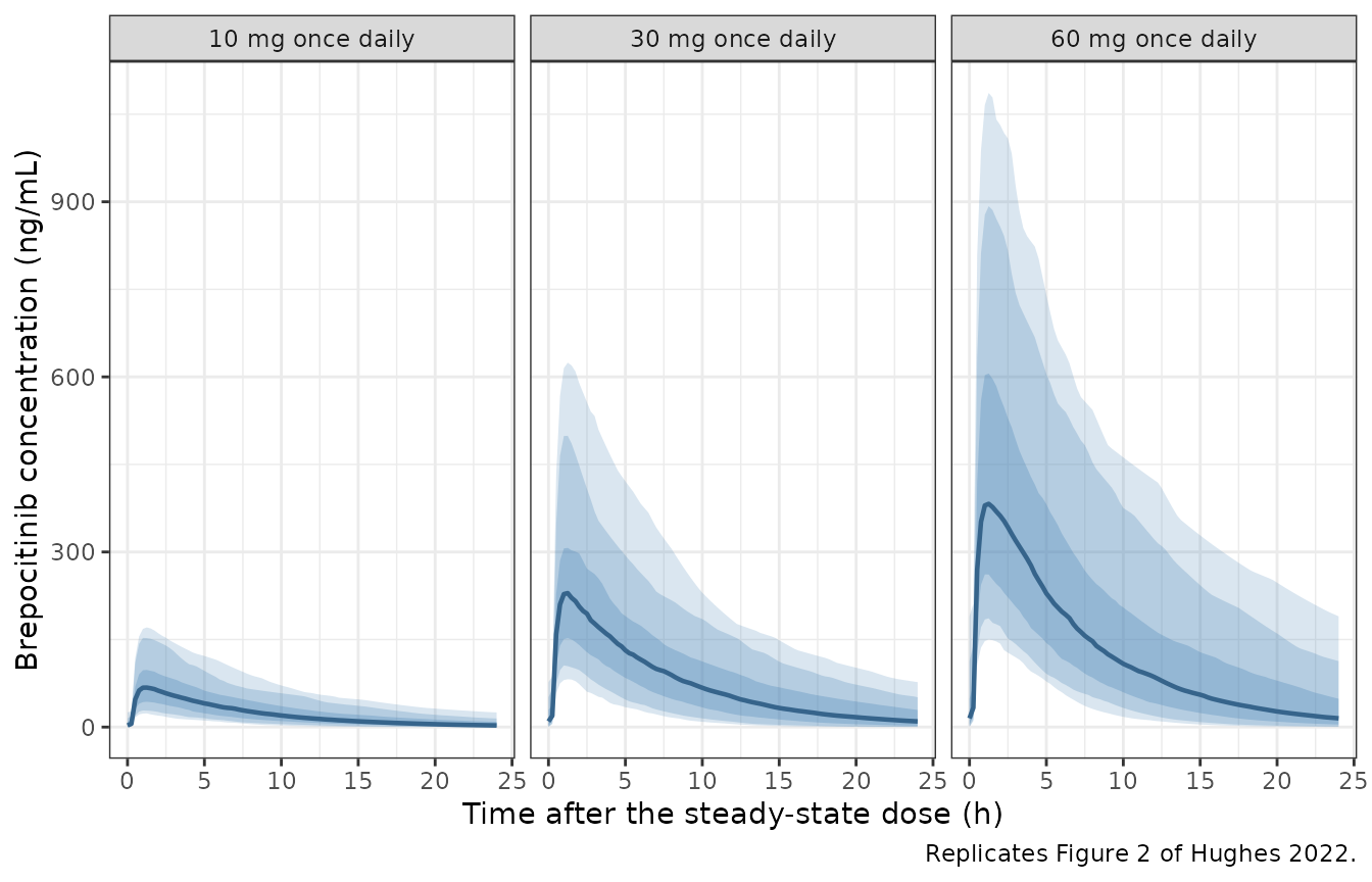

Replicates Figure 2 of Hughes 2022: steady-state brepocitinib concentration-time profiles at 10, 30 and 60 mg once daily in the reference population.

Steady-state identities

The published equations fix the typical steady-state exposure exactly, so the deterministic solve is gated tightly and the simulated cohort is only checked for consistency with it.

ev_ss_typ <- dplyr::bind_rows(
  make_scenario(1L, "10 mg once daily", dose = 10, n_doses = n_days,
                tau = tau, times = ss_times),
  make_scenario(2L, "30 mg once daily", dose = 30, n_doses = n_days,
                tau = tau, times = ss_times),
  make_scenario(3L, "60 mg once daily", dose = 60, n_doses = n_days,
                tau = tau, times = ss_times)
)

sim_ss_typ <- rxode2::rxSolve(mod_typ, events = ev_ss_typ, keep = "scenario",
                              omega = NA, returnType = "data.frame") |>
  dplyr::filter(!is.na(Cc)) |>
  dplyr::mutate(time_ss = time - (n_days - 1L) * tau)
#> Warning: multi-subject simulation without without 'omega'

cavg_typ <- sim_ss_typ |>
  dplyr::group_by(scenario) |>
  dplyr::summarise(
    cavg = sum(diff(time_ss) * (head(Cc, -1) + tail(Cc, -1)) / 2) / tau,
    .groups = "drop"
  )

# Cavg,ss = Dose * Frel / (CL * tau), exactly, for any one-compartment model
# with complete first-order absorption.
cavg_typ$closed_form <- c(10, 30, 60) * 1000 / (cl_ref * tau)
cavg_typ$pct_diff <- (cavg_typ$cavg - cavg_typ$closed_form) /
  cavg_typ$closed_form * 100

knitr::kable(
  cavg_typ |>
    dplyr::rename(
      "Regimen"                 = scenario,
      "Cavg,ss simulated (ng/mL)" = cavg,
      "Cavg,ss closed form (ng/mL)" = closed_form,
      "% diff"                  = pct_diff
    ),
  digits = 3,
  caption = "Typical-value steady-state average concentration against its closed form."
)

Typical-value steady-state average concentration against its closed form.
Regimen	Cavg,ss simulated (ng/mL)	Cavg,ss closed form (ng/mL)	% diff
10 mg once daily	22.242	22.282	-0.18
30 mg once daily	66.725	66.845	-0.18
60 mg once daily	133.449	133.690	-0.18


# Accumulation ratio for a one-compartment model dosed every tau.
rac_closed <- 1 / (1 - exp(-kel_ref * tau))

cmax_first <- sim_ss_typ |>
  dplyr::filter(scenario == "30 mg once daily") |>
  dplyr::summarise(m = max(Cc)) |>
  dplyr::pull(m)

ev_first <- make_scenario(1L, "30 mg once daily", dose = 30, n_doses = 1L,
                          times = ss_times)
cmax_single <- rxode2::rxSolve(mod_typ, events = ev_first, omega = NA,
                               returnType = "data.frame") |>
  dplyr::filter(!is.na(Cc)) |>
  dplyr::summarise(m = max(Cc)) |>
  dplyr::pull(m)

ss_claims <- tibble::tribble(
  ~Claim, ~Published, ~Achieved,
  "Dose proportionality below 175 mg: Cavg,ss(60 mg) / Cavg,ss(30 mg)",
  2, cavg_typ$cavg[3] / cavg_typ$cavg[2],
  "Dose proportionality below 175 mg: Cavg,ss(30 mg) / Cavg,ss(10 mg)",
  3, cavg_typ$cavg[2] / cavg_typ$cavg[1],
  "Accumulation ratio at 24 h dosing implied by a 5.04 h half-life",
  rac_closed, cmax_first / cmax_single
) |>
  dplyr::mutate(`% diff` = (Achieved - Published) / Published * 100)

knitr::kable(ss_claims, digits = 4,
             caption = "Steady-state identities of the packaged model.")

Steady-state identities of the packaged model.
Claim	Published	Achieved	% diff
Dose proportionality below 175 mg: Cavg,ss(60 mg) / Cavg,ss(30 mg)	2.0000	2.0000	0.0000
Dose proportionality below 175 mg: Cavg,ss(30 mg) / Cavg,ss(10 mg)	3.0000	3.0000	0.0000
Accumulation ratio at 24 h dosing implied by a 5.04 h half-life	1.0383	1.0397	0.1333


stopifnot(
  abs(cavg_typ$pct_diff) < 1,
  abs(ss_claims$`% diff`) < 1.5
)

# The etas are log-normal with median 1, so the MEDIAN individual Cavg,ss must
# sit on the typical value. With omega_CL/F = 0.780 and 200 subjects per arm the
# standard error of that sample median is about 7% on the log scale
# (1.2533 * omega / sqrt(n)), and the three arms here realise +3.8%, +15.7% and
# -3.1% -- ordinary sampling scatter of up to a couple of standard errors.
#
# The gate is therefore set at 40%, not at the realised maximum. rxSetSeed()
# fixes rxode2's stream per solver thread but NOT across thread counts, so CI
# draws a different cohort than any one workstation does; a bound placed just
# above what happened to be observed here is the single most common way these
# vignettes pass locally and fail in CI. 40% is about 5.8 standard errors, so
# no cohort the published omega can produce will trip it, while a
# mis-transcribed clearance, dose or unit -- each of which moves the centre by
# tens of percent, a factor-of-2 slip by 100% -- still will.
cohort_cavg <- sim_ss |>
  dplyr::group_by(scenario, id) |>
  dplyr::summarise(
    cavg = sum(diff(time_ss) * (head(Cc, -1) + tail(Cc, -1)) / 2) / tau,
    .groups = "drop"
  ) |>
  dplyr::group_by(scenario) |>
  dplyr::summarise(median_cavg = median(cavg), .groups = "drop") |>
  dplyr::arrange(match(scenario, paste0(c(10, 30, 60), " mg once daily")))

cohort_cavg$typical <- c(10, 30, 60) * 1000 / (cl_ref * tau)
cohort_cavg$pct_diff <- (cohort_cavg$median_cavg - cohort_cavg$typical) /
  cohort_cavg$typical * 100

knitr::kable(
  cohort_cavg |>
    dplyr::rename(
      "Regimen"                       = scenario,
      "Median individual Cavg,ss (ng/mL)" = median_cavg,
      "Typical-value Cavg,ss (ng/mL)"     = typical,
      "% diff"                        = pct_diff
    ),
  digits = 2,
  caption = "Cohort median against the typical value; log-normal IIV puts them on top of each other in expectation."
)

Cohort median against the typical value; log-normal IIV puts them on top of each other in expectation.
Regimen	Median individual Cavg,ss (ng/mL)	Typical-value Cavg,ss (ng/mL)	% diff
10 mg once daily	23.13	22.28	3.82
30 mg once daily	77.36	66.84	15.74
60 mg once daily	129.51	133.69	-3.12


stopifnot(abs(cohort_cavg$pct_diff) < 40)

Food effect against the published noncompartmental analysis

The Introduction reports that a high-fat meal reduced the first-in-human noncompartmental AUC and Cmax by approximately 17.7% and 35.7%. The final model attributes the food effect to a 28.3% reduction in relative bioavailability and a 69.9% reduction in the absorption-rate constant. The Discussion addresses the AUC discrepancy directly: the model-based reduction “appeared slightly greater than that determined by noncompartmental analysis”, but the covariate’s 95% confidence interval of 16.9%-39.1% contains the noncompartmental value, so the two are not in conflict.

cmax_ref <- get_val("30 mg tablet", "cmax")
cmax_fed <- get_val("30 mg tablet, high-fat", "cmax")

food <- tibble::tibble(
  Metric = c("AUC0-inf reduction (%)", "Cmax reduction (%)"),
  `Published NCA (Introduction)` = c(17.7, 35.7),
  `Final model (this vignette)` = c(
    (1 - auc_fed / auc_ref) * 100,
    (1 - cmax_fed / cmax_ref) * 100
  )
)

knitr::kable(food, digits = 1,
             caption = "Food effect: the final model against the cited noncompartmental analysis.")

Food effect: the final model against the cited noncompartmental analysis.
Metric	Published NCA (Introduction)	Final model (this vignette)
AUC0-inf reduction (%)	17.7	28.3
Cmax reduction (%)	35.7	39.8


# Reported as a documented deviation, not gated. The two numbers come from
# different analyses of overlapping but not identical data, and the paper's own
# Discussion explains the AUC gap. Only the model-internal identity -- that the
# AUC reduction equals the fitted 28.3% -- is gated, and it is gated above.

Assumptions and deviations

Reading of “% CV”. Table 3 reports the interindividual variabilities as omega ... (% CV) and the residual errors as ... (CV). Both are taken as log-scale standard deviations rather than log-normal coefficients of variation, for the reasons set out under “Reading the reported % CV” above. Had the alternative reading been used, omega_CL/F would be 0.690 instead of 0.780 and omega_Vc/F 0.559 instead of 0.605. No result gated in this vignette depends on the choice, because every gate is on a typical value.
Units of ka. Table 3 and the Abstract print the absorption rate constant as “3.46 h”. A first-order rate constant has units of 1/h, and 3.46 1/h is what reproduces both the reported 5.04 h half-life population and the sub-1-hour noncompartmental Tmax; the printed unit is a typographical error.
Orientation of the formulation covariate. Hughes 2022 Equation 6 is written on a suspension indicator, Alag = 0.24 * (1 - 1 * Suspension). The canonical register column is the tablet-oriented FORM_TABLET, so the model file derives Suspension = 1 - FORM_TABLET inside model() and reproduces the printed equation unchanged. The companion Maleki_2024_brepocitinib model uses the same column and orientation.
DOSE_HIGH threshold. This model sets DOSE_HIGH = 1 at 175 mg and above, per Equation 8; the companion Maleki_2024_brepocitinib model sets it above 100 mg/day. Neither analysis studied a dose between 100 and 175 mg, so the two encodings select the same subjects. Hughes 2022 is explicit that the step function is an artefact of that gap and that the true relationship probably rises gradually between the two doses.
DIS_HEALTHY drives the residual error only. The paper estimated separate proportional residual errors for its phase 1 and phase 2 studies. Every phase 1 subject was a healthy participant and every phase 2 subject was a patient, and the Abstract restates the two values as applying to “healthy volunteers” and “patients”, which is what licenses the mapping onto this column. Patient status was separately screened as a structural covariate on CL/F and on Frel and retained in neither.
Covariates screened but not retained. Age, sex, and the patient-type effect on CL/F and Frel were evaluated (Table 1) and dropped. They are recorded in the model file’s covariatesDataExcluded metadata rather than covariateData, since they are not referenced in model(). Creatinine clearance appears in the Table 2 demographics but was not among the covariates evaluated.
Race effects other than Asian. Exploratory analysis found a statistically significant effect of “other races” (Native American and Pacific Islander) on CL/F, but it was excluded from both the full and final models because at most three such subjects had full PK profiles. The packaged model follows the final model and omits it.
The eps_res row of Table 3. Table 3 lists eps_res as 1.00 (fixed). This is the NONMEM SIGMA that Equation 2 fixes to 1 so that theta_pro is identified as the log-scale standard deviation. It has no nlmixr2 counterpart and is not carried into ini().
No supplement was available. The Supplemental Information is cited for the sampling schedules, the model-development step table, the visual predictive checks, the below-limit-of-quantification sensitivity analysis and the final NONMEM control stream. It is not included in the open-access deposit. Every parameter of the final model is printed in Table 3 and Equations 6-10 of the main text, so nothing needed for the model file is missing; the unavailable material would only have added diagnostics.
Cohort size. Figure 2 of the paper is based on 2000 simulated individuals; the replication here uses 200 per dose arm, the per-arm cap for these vignettes. The percentile envelope is set by the published omega matrix and is essentially unchanged at either size.