Model and source
- Citation: Liva S, Chen M, Mortazavi A, Walker A, Wang J, Dittmar K, Hofmeister C, Coss CC, Phelps MA. Population Pharmacokinetic Analysis from First-in-Human Data for HDAC Inhibitor, REC-2282 (AR-42), in Patients with Solid Tumors and Hematologic Malignancies: A Case Study for Evaluating Flat vs. Body Size Normalized Dosing. Eur J Drug Metab Pharmacokinet. 2021;46:807-816. doi:10.1007/s13318-021-00722-z.
- Description: Two-compartment population PK model for the oral pan-histone-deacetylase inhibitor REC-2282 (AR-42) in 55 adults with relapsed or refractory solid tumours or haematologic malignancies pooled from the first-in-human trial OSU09102 (NCT01129193) and the phase 1 acute myeloid leukaemia trial OSU11130 (NCT01798901) (Liva 2021). Oral doses of 20-80 mg enter a depot after an absorption lag time and pass through one transit compartment to the central compartment, with the same first-order rate constant ka for both steps; elimination is first-order from the central compartment and all volumes and clearances are apparent (CL/F, Vc/F, Q/F, Vp/F). Fat-free mass (Janmahasatian) is a power covariate on CL/F centred on the cohort median of 50.8 kg, and tumour type (haematologic vs solid) and formulation (tablet vs capsule) are linear fractional covariates on the lag time. IIV on CL/F and ka; residual error is additive on log-transformed concentrations.
- Article: https://doi.org/10.1007/s13318-021-00722-z (open access; PMC8599380)
REC-2282 (development code AR-42, formerly OSU-HDAC42) is an oral pan-histone-deacetylase inhibitor with no international non-proprietary name, so the model is named for its current development code.
Population
Liva 2021 pooled two phase 1 trials run at The Ohio State University Comprehensive Cancer Center: the first-in-human trial OSU09102 (NCT01129193; multiple myeloma, lymphoma and advanced solid tumours including neurofibromatosis type 2) and OSU11130 (NCT01798901; relapsed or refractory acute myeloid leukaemia). Of 57 enrolled patients (44 + 13; Table 1), 882 plasma concentrations from 55 were modelled (Results 3.2). Table 2 summarises the 56 patients with anthropometric data: median weight 76.1 kg (42.9-122.4), median fat-free mass 50.8 kg (29.9-76.0), median BMI 26.0 kg/m^2, median age 63 years (20-80), 51.8% female. Supplemental Table 2 lists 40 patients with a haematologic malignancy (multiple myeloma 17, lymphoma 10, AML 13) and 16 with a solid tumour. Doses of 20-80 mg were taken fasted three times weekly (Monday, Wednesday, Friday; one OSU11130 cohort 40 mg four times weekly) for 3 weeks of each 28-day cycle, with intensive sampling on day 1 and on day 5 (OSU11130) or day 19 (OSU09102).
The same information is available programmatically via
readModelDb("Liva_2021_rec2282")()$population.
Source trace
Every ini() value carries an in-file comment pointing to
its source; the table collects them.
| Equation / parameter | Value | Source location |
|---|---|---|
| Structure: depot -(ka)-> transit -(ka)-> central <-> peripheral, lag on the dose | n/a | Fig. 2; Results 3.2; Discussion |
lcl (CL/F) |
log(11.6) L/h | Table 3, covariate model |
lvc (Vc/F) |
log(105) L | Table 3, covariate model |
lq (Q/F) |
log(7.1) L/h | Table 3, covariate model |
lvp (Vp/F) |
log(76.5) L | Table 3, covariate model |
lka (ka) |
log(1.28) 1/h | Table 3, covariate model |
ltlag (ALAG) |
log(0.0453) h | Table 3, covariate model (no IIV in the final model, Results 3.2) |
e_ffm_cl |
0.493 | Table 3 ‘Covariates FFM’; power form of Equation 1 |
e_heme_tlag |
0.942 | Table 3 ‘Covariates TMR’; linear form of Equation 2 |
e_tablet_tlag |
0.74 | Table 3 ‘Covariates FORM’; linear form of Equation 2 |
| FFM centring value | 50.8 kg | Table 2 median FFM, all patients; Section 2.3 (median normalisation) |
| FFM equation | Janmahasatian | Section 2.4 |
etalcl |
0.05068 | Table 3: 22.8 CV%, as log(CV^2 + 1) |
etalka |
0.20500 | Table 3: 47.7 CV%, as log(CV^2 + 1) |
expSd |
0.545 | Table 3 epsilon (SD, per footnote); Section 2.3 ‘additive error model for log-transformed data’ |
Virtual cohort
The observed data are not public. The virtual cohort reproduces the Table 2 demographics: body weight log-normal around the median of 76.1 kg, BMI normal with the Table 2 mean and SD, 51.8% female, and fat-free mass computed from these by the Janmahasatian equations the paper uses (Section 2.4). Tumour type follows the Supplemental Table 2 split (40 of 56 haematologic). The paper does not report how many patients took each formulation, so half the cohort is assigned capsules.
Four dose levels are simulated on the paper’s three-times-weekly schedule (doses on days 1, 3, 5, 8, 10, 12, 15, 17 and 19), with 100 virtual patients per arm.
set.seed(20211007)
dose_levels <- c(20, 40, 50, 60)
n_per_arm <- 100L

ffm_janmahasatian <- function(wt, bmi, sexf) {
  ifelse(
    sexf == 1,
    9270 * wt / (8780 + 244 * bmi),
    9270 * wt / (6680 + 216 * bmi)
  )
}

dose_days <- c(1, 3, 5, 8, 10, 12, 15, 17, 19)
dose_times <- (dose_days - 1) * 24
obs_rel <- c(0, 0.25, 0.5, 1, 1.5, 2, 3, 4, 6, 8, 10, 12, 16, 24)
obs_times <- sort(unique(c(
  obs_rel, 36, 47.99,          # day 1 (to the day 3 dose)
  96 + obs_rel,                # day 5
  432 + obs_rel, 432 + 36, 480 # day 19
)))

make_cohort <- function(n, dose, id_offset) {
  subj <- tibble(
    id = id_offset + seq_len(n),
    SEXF = rbinom(n, 1, 0.518),
    WT = pmin(pmax(exp(rnorm(n, log(76.1), 0.23)), 42.9), 122.4),
    BMI = pmin(pmax(rnorm(n, 26.7, 5.4), 18.5), 43.6),
    TUMTP_SOLID = 1L - rbinom(n, 1, 40 / 56),
    FORM_CAPSULE = rbinom(n, 1, 0.5),
    treatment = paste(dose, "mg")
  ) |>
    mutate(FFM = ffm_janmahasatian(WT, BMI, SEXF))
  doses <- tidyr::crossing(subj, time = dose_times) |>
    mutate(evid = 1L, amt = dose, cmt = "depot")
  obs <- tidyr::crossing(subj, time = obs_times) |>
    mutate(evid = 0L, amt = 0, cmt = "central")
  bind_rows(doses, obs) |>
    arrange(id, time, desc(evid))
}

events <- bind_rows(lapply(seq_along(dose_levels), function(i) {
  make_cohort(n_per_arm, dose_levels[i], id_offset = (i - 1L) * n_per_arm)
}))
stopifnot(!anyDuplicated(unique(events[, c("id", "time", "evid")])))

cohort <- distinct(events, id, treatment, SEXF, WT, BMI, FFM, TUMTP_SOLID)
summary(cohort$FFM)
#>    Min. 1st Qu.  Median    Mean 3rd Qu.    Max.
#>   24.80   43.69   50.41   52.49   59.53  106.28
The simulated median FFM (50.4 kg) lies close to the Table 2 median of 50.8 kg, so the virtual cohort is centred where the CL/F covariate term is anchored.
Simulation
mod <- readModelDb("Liva_2021_rec2282")
sim <- rxode2::rxSolve(
  mod,
  events = events,
  keep = c("treatment", "FFM", "TUMTP_SOLID", "FORM_CAPSULE")
) |>
  as.data.frame() |>
  mutate(
    day = case_when(
      time < 48 ~ "Day 1",
      time >= 96 & time <= 120 ~ "Day 5",
      time >= 432 ~ "Day 19",
      TRUE ~ NA_character_
    ),
    tad = case_when(
      day == "Day 1" ~ time,
      day == "Day 5" ~ time - 96,
      day == "Day 19" ~ time - 432
    )
  )
#> ℹ parameter labels from comments will be replaced by 'label()'
Cc is the individual prediction without residual
error.
Replicate published figures
# Replicates Figure 1 of Liva 2021: mean concentration by dose level on days 1, 5 and 19.
sim |>
  filter(!is.na(day)) |>
  group_by(day, treatment, time) |>
  summarise(Cc = mean(Cc), .groups = "drop") |>
  mutate(day = factor(day, c("Day 1", "Day 5", "Day 19"))) |>
  ggplot(aes(time, Cc, colour = treatment)) +
  geom_line() +
  facet_wrap(~day, ncol = 1, scales = "free_x") +
  scale_y_log10(limits = c(1, 1000)) +
  labs(
    x = "Time after first dose (h)", y = "REC-2282 (ng/mL)", colour = "Dose",
    caption = "Replicates Figure 1 of Liva 2021 (lines = mean of each dose group)."
  )
#> Warning in scale_y_log10(limits = c(1, 1000)): log-10 transformation introduced
#> infinite values.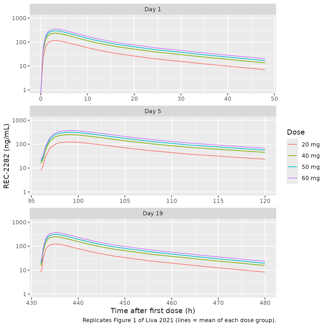
Figure 1 of the paper shows day-1 mean peaks of roughly 100 ng/mL at 20 mg to 300-400 ng/mL at 50-70 mg, falling to about 3-10 ng/mL by 48 h; the simulated means follow the same pattern.
# Replicates the style of Figure 3 of Liva 2021 (VPC) for the 40 mg arm, which
# contributed the most patients (Table 1).
set.seed(1)
sim |>
  filter(treatment == "40 mg", !is.na(day)) |>
  mutate(
    obs = Cc * exp(rnorm(n(), 0, 0.545)),
    day = factor(day, c("Day 1", "Day 5", "Day 19"))
  ) |>
  group_by(day, tad) |>
  summarise(
    Q05 = quantile(obs, 0.05), Q50 = quantile(obs, 0.50),
    Q95 = quantile(obs, 0.95), .groups = "drop"
  ) |>
  ggplot(aes(tad, Q50)) +
  geom_ribbon(aes(ymin = Q05, ymax = Q95), alpha = 0.25) +
  geom_line() +
  facet_wrap(~day) +
  scale_y_log10() +
  labs(
    x = "Time after dose (h)", y = "REC-2282 (ng/mL)",
    caption = "Simulated 5th/50th/95th percentiles with residual error, 40 mg arm (cf. Figure 3 of Liva 2021)."
  )
#> Warning in scale_y_log10(): log-10 transformation introduced infinite values.
#> log-10 transformation introduced infinite values.
#> log-10 transformation introduced infinite values.
#> log-10 transformation introduced infinite values.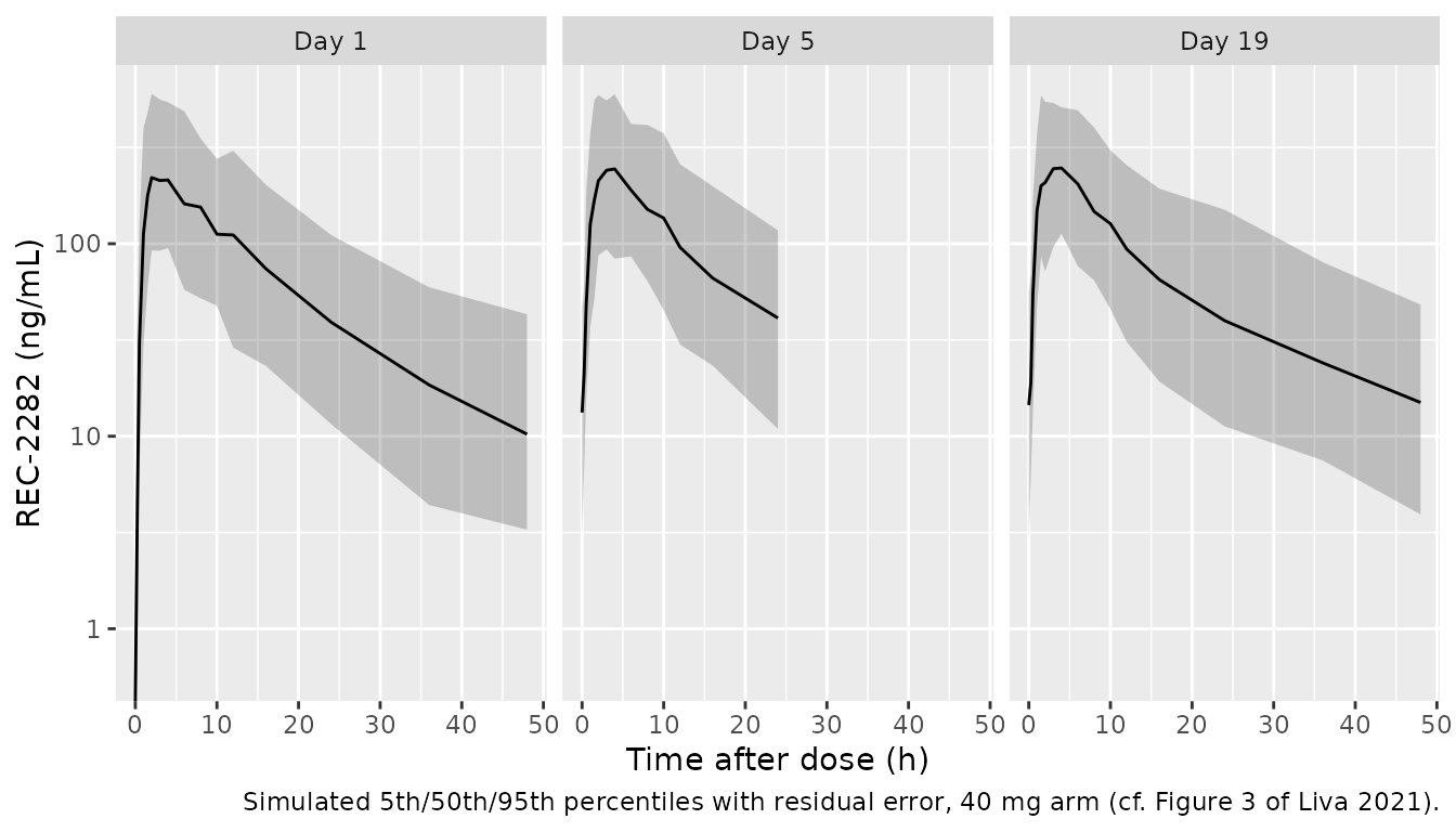
Supplemental Figure 3: typical AUC at a 40 mg flat dose
Supplemental Figure 3 shows simulated AUCs for the patients dosed at 40 mg flat. The box is narrow (whiskers about 2.7-3.2 hmg/L, median about 2.85 hmg/L), which indicates typical-value predictions that vary only by each patient’s FFM. The paper does not state the AUC window, so the typical-value AUC over 0-24 h, 0-48 h (the dosing interval) and 0-infinity is shown for the cohort median FFM.
mod_typ <- rxode2::zeroRe(mod)
#> ℹ parameter labels from comments will be replaced by 'label()'
ev_typ <- rxode2::et(amt = 40, cmt = "depot") |>
  rxode2::et(seq(0, 480, by = 0.05), cmt = "central") |>
  as.data.frame() |>
  mutate(FFM = 50.8, TUMTP_SOLID = 1, FORM_CAPSULE = 1)
typ <- as.data.frame(rxode2::rxSolve(mod_typ, ev_typ))
#> ℹ omega/sigma items treated as zero: 'etalcl', 'etalka'
trap <- function(t, y) sum(diff(t) * (head(y, -1) + tail(y, -1)) / 2)
auc_window <- function(end) {
  x <- typ[typ$time <= end, ]
  trap(x$time, x$Cc) / 1000
}
typ_auc <- tibble(
  window = c("0-24 h", "0-48 h", "0-infinity (dose / CL)"),
  auc = c(auc_window(24), auc_window(48), 40 / 11.6)
)
knitr::kable(
  typ_auc |> rename("AUC window" = window, "Typical AUC (h*mg/L)" = auc),
  digits = 2,
  caption = "Typical-value AUC after 40 mg at FFM = 50.8 kg; Supplemental Figure 3 median is about 2.85 h*mg/L."
)| AUC window | Typical AUC (h*mg/L) |
|---|---|
| 0-24 h | 2.64 |
| 0-48 h | 3.18 |
| 0-infinity (dose / CL) | 3.45 |
# Structural gate: the digitised median (2.85) must lie between the shortest
# and the longest plausible window. A mis-transcribed CL or unit moves both
# bounds by the same factor and breaks this.
stopifnot(typ_auc$auc[1] < 2.85 * 1.1, typ_auc$auc[3] > 2.85 * 0.9)
The digitised median of 2.85 h*mg/L falls between the typical AUC0-24 and the AUC0-infinity. (The trapezoid sum above is a check on a single noiseless profile; the cohort NCA below uses PKNCA.)
PKNCA validation
NCA is run on the day-1 and day-19 dosing days over 0-24 h after the dose, per dose level.
sim_nca <- sim |>
  filter(!is.na(Cc), day %in% c("Day 1", "Day 19"), tad <= 24) |>
  select(id, time, Cc, treatment)

conc_obj <- PKNCA::PKNCAconc(sim_nca, Cc ~ time | treatment + id)
dose_df <- events |>
  filter(evid == 1) |>
  select(id, time, amt, treatment)
dose_obj <- PKNCA::PKNCAdose(dose_df, amt ~ time | treatment + id)

intervals <- data.frame(
  start = c(0, 432),
  end = c(24, 456),
  cmax = TRUE,
  tmax = TRUE,
  auclast = TRUE
)
nca_res <- PKNCA::pk.nca(PKNCA::PKNCAdata(conc_obj, dose_obj, intervals = intervals))

nca_df <- as.data.frame(nca_res$result) |>
  mutate(day = ifelse(start == 0, "Day 1", "Day 19"))

nca_df |>
  filter(PPTESTCD %in% c("cmax", "tmax", "auclast")) |>
  group_by(treatment, day, PPTESTCD) |>
  summarise(median = median(PPORRES), .groups = "drop") |>
  tidyr::pivot_wider(names_from = PPTESTCD, values_from = median) |>
  rename(
    "Dose" = treatment, "Day" = day, "Cmax (ng/mL)" = cmax,
    "Tmax (h)" = tmax, "AUC0-24 (ng*h/mL)" = auclast
  ) |>
knitr::kable(digits = 1, caption = "Simulated median NCA by dose level and day.")| Dose | Day | AUC0-24 (ng*h/mL) | Cmax (ng/mL) | Tmax (h) |
|---|---|---|---|---|
| 20 mg | Day 1 | 1322.2 | 126.9 | 3 |
| 20 mg | Day 19 | 1423.1 | 135.7 | 3 |
| 40 mg | Day 1 | 2629.5 | 257.0 | 3 |
| 40 mg | Day 19 | 2827.4 | 268.3 | 3 |
| 50 mg | Day 1 | 3304.6 | 315.2 | 3 |
| 50 mg | Day 19 | 3576.4 | 331.4 | 3 |
| 60 mg | Day 1 | 3856.0 | 380.5 | 3 |
| 60 mg | Day 19 | 4137.1 | 401.3 | 3 |
Comparison against published NCA
Liva 2021 does not tabulate NCA. The first-in-human report of the haematologic arm of OSU09102 (Sborov et al., Leuk Lymphoma 2017;58:2310-2318, doi:10.1080/10428194.2017.1298751) gives day-1 and day-19 geometric-mean Cmax of 0.383 and 0.335 uM at 20 mg, 0.794 and 0.830 uM at 40 mg, and 1.60 and 1.50 uM at 50 mg. These are converted to ng/mL with the REC-2282 molecular weight of 312.4 g/mol (C18H20N2O3). The simulated median is compared with the geometric mean, which is close to the median for log-normal data.
mw <- 312.37
published <- tibble::tribble(
  ~treatment, ~day, ~cmax,
  "20 mg", "Day 1", 0.383,
  "20 mg", "Day 19", 0.335,
  "40 mg", "Day 1", 0.794,
  "40 mg", "Day 19", 0.830,
  "50 mg", "Day 1", 1.60,
  "50 mg", "Day 19", 1.50
) |>
  mutate(cmax = cmax * mw)

cmp <- nlmixr2lib::ncaComparisonTable(
  simulated = nca_df |> filter(treatment %in% published$treatment),
  reference = published,
  by = c("treatment", "day"),
  params = "cmax",
  units = c(cmax = "ng/mL"),
  tolerance_pct = 20
)
knitr::kable(cmp, caption = "Simulated vs. published Cmax (Sborov 2017). * differs by >20%.")| NCA parameter | treatment | day | Reference | Simulated | % diff |
|---|---|---|---|---|---|
| Cmax (ng/mL) | 20 mg | Day 1 | 120 | 127 | +6.1% |
| Cmax (ng/mL) | 20 mg | Day 19 | 105 | 136 | +29.7%* |
| Cmax (ng/mL) | 40 mg | Day 1 | 248 | 257 | +3.6% |
| Cmax (ng/mL) | 40 mg | Day 19 | 259 | 268 | +3.5% |
| Cmax (ng/mL) | 50 mg | Day 1 | 500 | 315 | -36.9%* |
| Cmax (ng/mL) | 50 mg | Day 19 | 469 | 331 | -29.3%* |
The 40 mg arm agrees within 5% on both days, as does day 1 at 20 mg. The flagged 20 mg day-19 row reflects a published day-19 value below the day-1 value in a three-patient arm; the linear model predicts slight accumulation instead. The 50 mg arm of Sborov 2017 had geometric-mean Cmax values about double those at 40 mg, which is more than dose proportional. Liva 2021 reports dose-proportional PK across 20-80 mg in the pooled data (Discussion), so the model, which is linear, falls short of that small arm by roughly the dose ratio. The 40 mg arm has the most patients and is used as the gate:
cmax40 <- nca_df |>
  filter(treatment == "40 mg", PPTESTCD == "cmax")
# Centre gate: a mis-transcribed Vc, ka or dose unit shifts the median Cmax by
# tens of percent. Robust to which subjects land in the tails.
stopifnot(abs(median(cmax40$PPORRES) / (0.794 * mw) - 1) < 0.2)

# Variability gate. The Discussion reports that observed dose-normalised AUC
# varied by 24.1%. The simulated between-subject CV of AUC0-24 comes from IIV on
# CL/F (22.8% CV) and ka plus the FFM effect. It sits somewhat lower (about
# 15-17% per arm when this vignette was written) because a 24 h window is less
# sensitive to CL/F than AUC0-infinity and the observed value also carries assay
# noise. The bounds are an envelope, not a match, and were checked to go red:
# with the IIV removed the CV falls to about 8%, and reading the Table 3 CV% as
# a variance (omega^2 = 0.228, 0.477) raises it to about 28%.
auc_d1 <- nca_df |> filter(PPTESTCD == "auclast", day == "Day 1")
cv_auc <- auc_d1 |>
  group_by(treatment) |>
  summarise(cv = sd(PPORRES) / mean(PPORRES) * 100, .groups = "drop")
cv_auc
#> # A tibble: 4 × 2
#>   treatment    cv
#>   <chr>     <dbl>
#> 1 20 mg      16.6
#> 2 40 mg      15.6
#> 3 50 mg      14.9
#> 4 60 mg      15.2
stopifnot(median(cv_auc$cv) > 11, median(cv_auc$cv) < 22)
Covariate effects on the lag time
tibble(
  group = c(
    "Solid tumour, capsule", "Solid tumour, tablet",
    "Haematologic, capsule", "Haematologic, tablet"
  ),
  TUMTP_SOLID = c(1, 1, 0, 0),
  FORM_CAPSULE = c(1, 0, 1, 0)
) |>
  mutate(alag_min = 60 * 0.0453 * (1 + 0.942 * (1 - TUMTP_SOLID)) * (1 + 0.74 * (1 - FORM_CAPSULE))) |>
  select(group, alag_min) |>
  rename("Group" = group, "Typical lag time (min)" = alag_min) |>
knitr::kable(digits = 1)| Group | Typical lag time (min) |
|---|---|
| Solid tumour, capsule | 2.7 |
| Solid tumour, tablet | 4.7 |
| Haematologic, capsule | 5.3 |
| Haematologic, tablet | 9.2 |
The lag time is 3-9 minutes in every group, which is short against the absorption half-life of about 30 minutes (ln 2 / 1.28 1/h, through two compartments). The tumour-type and formulation effects therefore barely change the simulated profiles.
Assumptions and deviations
-
Coding of the tumour-type and formulation
covariates. Liva 2021 evaluates tumour type ‘as dichotomous
variables for solid vs. heme tumor’ and defines FORM as ‘formulation
(capsule vs. tablet)’, but never says which level is coded 1. It has no
reference-subject statement, no control stream, and no supplement table
that settles it. The maintainers took the first-named level as the
reference (0): solid tumour for tumour type and capsule for formulation.
So haematologic malignancy and the tablet carry the fractional increases
of 0.942 and 0.74 on ALAG. The model expresses both through the existing
canonical indicators, whose value 1 marks the reference level here:
ALAG = 0.0453 * (1 + 0.942 * (1 - TUMTP_SOLID)) * (1 + 0.74 * (1 - FORM_CAPSULE)). With the opposite coding, the typical lag would sit with haematologic patients on tablets instead. The practical effect is small because every group’s typical lag is under 10 minutes. - Formulation mix. The paper does not report which patients took capsules or tablets; the virtual cohort assigns 50% to each.
-
IIV scale. Table 3 reports IIV as CV%. The
variances use
omega^2 = log(CV^2 + 1), which is appropriate for the exponential IIV model in Section 2.3. Reading the CV assqrt(omega^2)instead would change the variances by 4% (CL) and 10% (ka). -
Residual error. Table 3 labels epsilon
‘proportional’, while Section 2.3 describes an ‘additive error model for
log-transformed data’. The two are the same model on the linear scale,
encoded here as a log-normal residual with
expSd = 0.545(an SD, per the Table 3 footnote). -
Lag placement. The Discussion says the lag was
added ‘into the transit compartment’, while Fig. 2 draws it on the oral
dose entering the depot. For a linear chain the two are equivalent (the
input is simply delayed); the model applies
alag(depot). - FFM centring. Section 2.3 normalises continuous covariates by the population median. The Table 2 median over the 56 patients with anthropometrics (50.8 kg) is used; the modelled population was 55 patients.
- Non-paper-derived values in this vignette. The external Cmax comparison uses Sborov et al. 2017 (the OSU09102 haematologic cohort) and the REC-2282 molecular weight of 312.4 g/mol (C18H20N2O3). Neither enters the model.
- No erratum or correction notice for Liva 2021 was found on Crossref or Europe PMC (checked 2026-09-29).