Ropeginterferon alfa-2b (Zhu 2021) • nlmixr2lib

Model and source

Citation: Zhu M, Wang M-X, Li Z-R, Wang W, Su X, Jiao Z. Population Pharmacokinetics of Ropeginterferon Alfa-2b: A Comparison Between Healthy Caucasian and Chinese Subjects. Front Pharmacol. 2021;12:673492. doi:10.3389/fphar.2021.673492.
Description: One-compartment quasi-equilibrium target-mediated drug disposition (QE-TMDD) population pharmacokinetic model for subcutaneous ropeginterferon alfa-2b (a mono-PEGylated interferon alfa-2b) in 57 healthy adult volunteers pooled from two single-dose phase I studies: 30 Caucasian men (A09-102, 24-270 ug) and 27 Chinese men and women (A17-101, 90-270 ug). First-order absorption with a lag time into a single serum compartment carrying linear clearance plus saturable binding (KD) to a turnover receptor pool (R0, kdeg), with the drug-receptor complex internalised at kint. Body weight acts on the linear clearance as a power function referenced to 70 kg; ethnicity had no significant effect.
Article (open access): https://doi.org/10.3389/fphar.2021.673492
Supplementary Material (Supplementary Tables 1-3, one DOCX): available from the article landing page and from Europe PMC under PMC8193675.

Zhu 2021 is the first population PK model of ropeginterferon alfa-2b. It pools two single-dose phase I studies in healthy volunteers to ask whether the PK differs between Caucasian and Chinese subjects, and concludes it does not once body weight is accounted for. A later analysis of the same drug in Chinese and Japanese patients with polycythaemia vera, with the same quasi-equilibrium TMDD structure, is packaged as Qin_2025_ropeginterferon.

Population

Fifty-seven healthy adults contributed 894 serum concentrations (Zhu 2021 Table 1):

Study A09-102 (Montreal, Canada): 30 Caucasian men given a single subcutaneous dose of 24, 48, 90, 180, 225 or 270 ug; body weight 79.4 +/- 9.41 kg; 456 observations.
Study A17-101 (Beijing, China): 27 Chinese adults (15 men, 12 women) given a single subcutaneous dose of 90, 180 or 270 ug; body weight 68.1 +/- 10 kg; 438 observations.

Ages were 18-45 years by protocol (mean 32.3 years). Sampling ran from pre-dose to 672 h. Nine subjects (six Caucasian, three Chinese) were excluded for drop-out.

str(readModelDb("Zhu_2021_ropeginterferon")()$population)
#> List of 12
#>  $ species       : chr "human"
#>  $ n_subjects    : int 57
#>  $ n_studies     : int 2
#>  $ n_observations: int 894
#>  $ age_range     : chr "18-45 years by protocol; mean 32.3 +/- 6.52 (Zhu 2021 Table 1)"
#>  $ weight_range  : chr "mean 74 +/- 11.2 kg pooled; Caucasian 79.4 +/- 9.41, Chinese 68.1 +/- 10 (Zhu 2021 Table 1)"
#>  $ sex_female_pct: num 21.1
#>  $ race_ethnicity: chr "Caucasian 30 (52.6%, all male, A09-102, Canada); Chinese 27 (47.4%, 15 male / 12 female, A17-101, Beijing)"
#>  $ disease_state : chr "Healthy volunteers"
#>  $ dose_range    : chr "Single subcutaneous dose: 24, 48, 90, 180, 225 or 270 ug (A09-102, six per cohort before drop-out) and 90, 180 "| __truncated__
#>  $ regions       : chr "Canada (Montreal) and China (Beijing)"
#>  $ notes         : chr "66 subjects received ropeginterferon alfa-2b; 9 (6 Caucasian, 3 Chinese) were excluded for drop-out, leaving 57"| __truncated__

Source trace

Every ini() value carries an in-file comment pointing to its source. The table collects them.

Equation / parameter	Value	Source location
`lka`	log(0.14 / 24) 1/h	Table 2, ka 0.14 1/day
`ltlag`	log(0.426) h	Table 2, tlag 0.426 h
`lcl`	log(0.778 / 24) L/h	Table 2, CL/F 0.778 L/day (70 kg)
`lvc`	log(2.32) L	Table 2, V/F
`lrbase`	log(0.111) ng/mL	Table 2, R0
`lkint`	fixed(log(0.0788)) 1/h	Table 2 (Fixed); Results, Base Model
`lkdeg`	log(0.544) 1/h	Table 2, kdeg
`lkd`	fixed(log(0.142)) ng/mL	Table 2 (Fixed); Results, Base Model
`e_wt_cl`	0.927	Table 2 ‘Impact of body weight’; Equation 15
`etalcl`, `etalvc`, `etalka`	35.7%, 90.8%, 63.5% CV	Table 2, Between subject variability
`propSd`, `addSd`	0.187, 0.342 ng/mL	Table 2, Residual unexplained variability; Equation 12
`d/dt(depot)`		Equation 2
`d/dt(central)` (total drug)		Equation 3
`d/dt(total_target)`		Equation 4
`total_target(0) = R0`, `ksyn = R0 * kdeg`		Equation 5; Figure 1B
free drug `cfree`		Equation 6
`CL/F = 0.778 * (WT/70)^0.927`		Equation 15

Unit check: kint and kdeg are per hour

Table 2 prints CL/F (L/day) and ka (1/day) in days but tlag, kint and kdeg in hours, and Supplementary Table 2 repeats exactly the same mix. The two readings of the target-mediated rates give very different models, so the choice is tested here against the paper’s own noncompartmental analysis (Supplementary Table 1, arithmetic means of the observed data) with a deterministic typical-value solve at the Caucasian mean weight.

mod <- readModelDb("Zhu_2021_ropeginterferon")
mod_typ <- mod |> rxode2::zeroRe()

typical_auc <- function(m, doses, wt) {
  ev <- dplyr::bind_rows(
    tibble::tibble(id = seq_along(doses), time = 0, evid = 1L, amt = doses, cmt = "depot"),
    tidyr::expand_grid(id = seq_along(doses), time = seq(0, 2000, by = 1)) |>
      dplyr::mutate(evid = 0L, amt = 0, cmt = "central")
  ) |>
    dplyr::arrange(id, time, dplyr::desc(evid)) |>
    dplyr::mutate(WT = wt)
  s <- rxode2::rxSolve(m, ev, returnType = "data.frame")
  s |>
    dplyr::filter(!is.na(Cc)) |>
    dplyr::distinct(id, time, .keep_all = TRUE) |>
    dplyr::group_by(id) |>
    dplyr::summarise(
      auc = sum(diff(time) * (head(Cc, -1) + tail(Cc, -1)) / 2),
      cmax = max(Cc),
      .groups = "drop"
    ) |>
    dplyr::mutate(dose = doses)
}

doses_cau <- c(24, 48, 90, 180, 225, 270)
nca_cau <- c(373.97, 620.61, 1243.54, 3891.48, 4352.23, 6184.44)

per_hour <- typical_auc(mod_typ, doses_cau, wt = 79.4)
# The alternative reading: kint and kdeg per day, i.e. 24-fold slower.
mod_day <- mod_typ |>
  rxode2::ini(lkint = log(0.0788 / 24), lkdeg = log(0.544 / 24))
per_day <- typical_auc(mod_day, doses_cau, wt = 79.4)

unit_tab <- tibble::tibble(
  dose = doses_cau,
  nca_mean = nca_cau,
  per_hour = per_hour$auc,
  per_day = per_day$auc
) |>
  dplyr::mutate(
    pct_hour = 100 * (per_hour - nca_mean) / nca_mean,
    pct_day = 100 * (per_day - nca_mean) / nca_mean
  )
unit_tab |>
  dplyr::rename(
    "Dose (ug)" = dose,
    "NCA mean AUC0-inf (ng*h/mL)" = nca_mean,
    "kint/kdeg per hour" = per_hour,
    "kint/kdeg per day" = per_day,
    "% diff, per hour" = pct_hour,
    "% diff, per day" = pct_day
  ) |>
  knitr::kable(digits = 0, caption = "Typical-value AUC0-inf at 79.4 kg against the Supplementary Table 1 Caucasian NCA means.")

Typical-value AUC0-inf at 79.4 kg against the Supplementary Table 1 Caucasian NCA means.
Dose (ug)	NCA mean AUC0-inf (ng*h/mL)	kint/kdeg per hour	kint/kdeg per day	% diff, per hour	% diff, per day
24	374	276	810	-26	116
48	621	646	1523	4	145
90	1244	1472	2729	18	119
180	3891	3563	5262	-8	35
225	4352	4677	6518	7	50
270	6184	5813	7770	-6	26


# Dose-normalised exposure rises from 24 to 270 ug in the observed NCA
# (22.9 vs 15.6 ng*h/mL per ug, ratio 1.47) because the target-mediated
# arm saturates. Only the per-hour reading reproduces that (ratio ~1.9);
# read per day, the target arm is negligible and the ratio falls below 1.
nonlin <- function(x) (x$auc[6] / 270) / (x$auc[1] / 24)
c(per_hour = nonlin(per_hour), per_day = nonlin(per_day))
#>  per_hour   per_day 
#> 1.8697105 0.8532263
stopifnot(
  nonlin(per_hour) > 1.3,
  nonlin(per_day) < 1.1,
  # The per-hour reading stays within 30% of every observed mean; the
  # per-day reading overpredicts the three lowest doses more than 2-fold.
  all(abs(unit_tab$pct_hour) < 30),
  all(unit_tab$pct_day[1:3] > 100)
)

The per-hour reading reproduces the observed greater-than-proportional rise in dose-normalised exposure (ratio about 1.9 against the observed 1.47) and lands within 30% of every observed mean AUC, each of which comes from about five subjects. The per-day reading overpredicts the three lowest doses by more than 100%. The model is therefore run in hours with kint, kdeg and tlag as printed and CL/F and ka divided by 24.

Virtual cohort

Nine arms reproduce the study design: six Caucasian dose groups and three Chinese dose groups, 100 subjects each. Body weight is drawn from a normal distribution with the Table 1 mean and SD of each study, redrawn (not clamped) outside 45-120 kg.

set.seed(2021)

draw_wt <- function(n, mean, sd) {
  wt <- rnorm(n, mean, sd)
  bad <- wt < 45 | wt > 120
  while (any(bad)) {
    wt[bad] <- rnorm(sum(bad), mean, sd)
    bad <- wt < 45 | wt > 120
  }
  wt
}

obs_times <- c(0, 1, 3, 6, 9, 12, 16, 24, 36, 48, 72, 96, 120, 144, 168,
               192, 240, 288, 336, 504, 672)

make_arm <- function(n, dose, pop, wt_mean, wt_sd, id_offset) {
  ids <- id_offset + seq_len(n)
  wt <- draw_wt(n, wt_mean, wt_sd)
  dose_rows <- tibble::tibble(id = ids, time = 0, evid = 1L, amt = dose, cmt = "depot")
  obs_rows <- tidyr::expand_grid(id = ids, time = obs_times) |>
    dplyr::mutate(evid = 0L, amt = 0, cmt = "central")
  dplyr::bind_rows(dose_rows, obs_rows) |>
    dplyr::left_join(tibble::tibble(id = ids, WT = wt), by = "id") |>
    dplyr::mutate(
      population = pop,
      dose = dose,
      treatment = paste0(pop, " ", dose, " ug")
    ) |>
    dplyr::arrange(id, time, dplyr::desc(evid))
}

arms <- tibble::tribble(
  ~pop,        ~dose, ~wt_mean, ~wt_sd,
  "Caucasian",    24,     79.4,   9.41,
  "Caucasian",    48,     79.4,   9.41,
  "Caucasian",    90,     79.4,   9.41,
  "Caucasian",   180,     79.4,   9.41,
  "Caucasian",   225,     79.4,   9.41,
  "Caucasian",   270,     79.4,   9.41,
  "Chinese",      90,     68.1,  10,
  "Chinese",     180,     68.1,  10,
  "Chinese",     270,     68.1,  10
)
n_per_arm <- 100L
events <- dplyr::bind_rows(lapply(seq_len(nrow(arms)), function(i) {
  make_arm(n_per_arm, arms$dose[i], arms$pop[i], arms$wt_mean[i], arms$wt_sd[i],
           id_offset = (i - 1L) * n_per_arm)
}))
stopifnot(!anyDuplicated(unique(events[, c("id", "time", "evid")])))

Simulation

sim <- rxode2::rxSolve(mod, events = events,
                       keep = c("population", "dose", "treatment", "WT")) |>
  as.data.frame()
#> ℹ parameter labels from comments will be replaced by 'label()'

Replicate published figures

Figure 2: concentration-time profiles by dose

sim |>
  dplyr::filter(time > 0) |>
  dplyr::group_by(population, dose, time) |>
  dplyr::summarise(
    Q10 = quantile(Cc, 0.10), Q50 = median(Cc), Q90 = quantile(Cc, 0.90),
    .groups = "drop"
  ) |>
  dplyr::mutate(dose = factor(paste(dose, "ug"), levels = paste(doses_cau, "ug"))) |>
  ggplot(aes(time, Q50, colour = population, fill = population)) +
  geom_ribbon(aes(ymin = Q10, ymax = Q90), alpha = 0.2, colour = NA) +
  geom_line() +
  facet_wrap(~dose) +
  scale_y_log10() +
  labs(x = "Time (h)", y = "Total serum ropeginterferon alfa-2b (ng/mL)",
       colour = NULL, fill = NULL,
       caption = "Median and 10th-90th percentiles of the simulation. Compare Figure 2B of Zhu 2021.")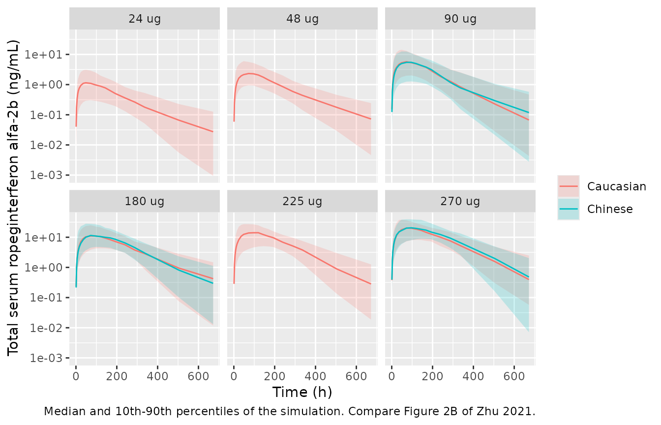

Figure 3: apparent clearance falls with dose

Figure 3 of Zhu 2021 plots NCA CL/F (L/h) against dose; the fitted trend falls from about 0.078 L/h at 24 ug to about 0.05 L/h at 270 ug in Caucasians and from about 0.07 to 0.04 L/h in Chinese subjects.

sim_nca <- sim |>
  dplyr::filter(!is.na(Cc)) |>
  dplyr::select(id, time, Cc, treatment)
sim_nca <- dplyr::bind_rows(
  sim_nca,
  sim_nca |> dplyr::distinct(id, treatment) |> dplyr::mutate(time = 0, Cc = 0)
) |>
  dplyr::distinct(id, treatment, time, .keep_all = TRUE) |>
  dplyr::arrange(id, treatment, time)

dose_df <- events |>
  dplyr::filter(evid == 1) |>
  dplyr::select(id, time, amt, treatment)

conc_obj <- PKNCA::PKNCAconc(sim_nca, Cc ~ time | treatment + id,
                             concu = "ng/mL", timeu = "h")
dose_obj <- PKNCA::PKNCAdose(dose_df, amt ~ time | treatment + id, doseu = "ug")
intervals <- data.frame(start = 0, end = Inf, cmax = TRUE, tmax = TRUE,
                        auclast = TRUE, aucinf.obs = TRUE, half.life = TRUE)
nca_res <- PKNCA::pk.nca(PKNCA::PKNCAdata(conc_obj, dose_obj, intervals = intervals))

nca_ind <- as.data.frame(nca_res) |>
  dplyr::filter(PPTESTCD %in% c("cmax", "auclast", "aucinf.obs")) |>
  dplyr::select(treatment, id, PPTESTCD, PPORRES) |>
  tidyr::pivot_wider(names_from = PPTESTCD, values_from = PPORRES) |>
  dplyr::left_join(dplyr::distinct(dose_df, id, amt), by = "id") |>
  dplyr::left_join(dplyr::distinct(sim, id, population), by = "id") |>
  # ug / (ng*h/mL) = L/h
  dplyr::mutate(clf = amt / aucinf.obs)

nca_ind |>
  ggplot(aes(amt, clf, colour = population)) +
  geom_point(alpha = 0.15, position = position_jitter(width = 3)) +
  stat_summary(fun = median, geom = "line", linewidth = 1) +
  facet_wrap(~population) +
  scale_x_continuous(breaks = doses_cau) +
  coord_cartesian(ylim = c(0, 0.2)) +
  labs(x = "Dose (ug)", y = "CL/F = Dose / AUC0-inf (L/h)", colour = NULL,
       caption = "Simulated subjects; line = median by dose. Compare Figure 3 of Zhu 2021.")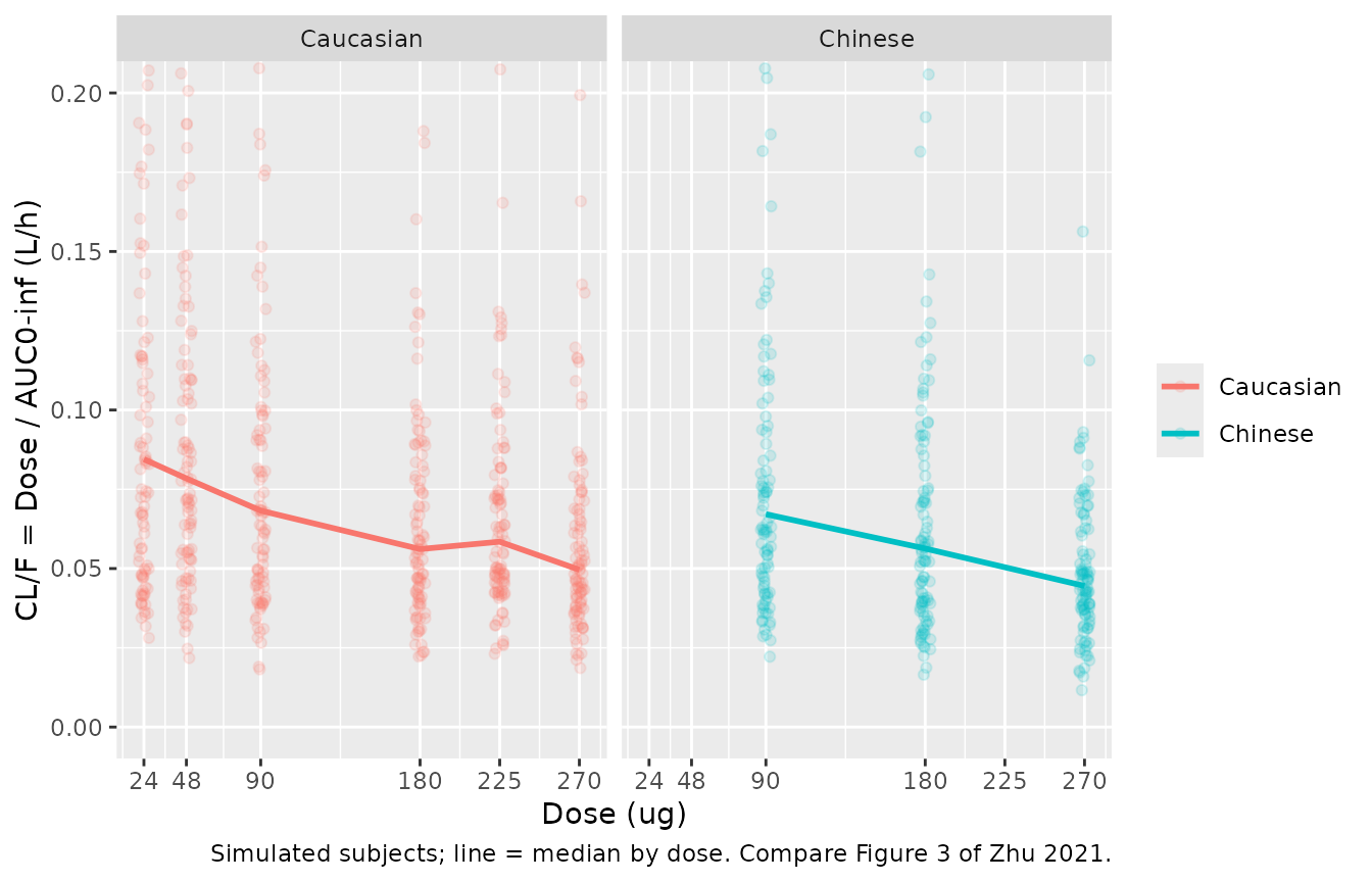


clf_med <- nca_ind |>
  dplyr::group_by(population, amt) |>
  dplyr::summarise(clf = median(clf), .groups = "drop")
clf_med
#> # A tibble: 9 × 3
#>   population   amt    clf
#>   <chr>      <dbl>  <dbl>
#> 1 Caucasian     24 0.0845
#> 2 Caucasian     48 0.0784
#> 3 Caucasian     90 0.0683
#> 4 Caucasian    180 0.0561
#> 5 Caucasian    225 0.0585
#> 6 Caucasian    270 0.0496
#> 7 Chinese       90 0.0671
#> 8 Chinese      180 0.0563
#> 9 Chinese      270 0.0445
stopifnot(
  # The saturable target arm makes CL/F fall with dose in both populations.
  with(clf_med, clf[population == "Caucasian" & amt == 24] /
         clf[population == "Caucasian" & amt == 270]) > 1.3,
  with(clf_med, clf[population == "Chinese" & amt == 90] /
         clf[population == "Chinese" & amt == 270]) > 1.1
)

Comparison against the published NCA (Supplementary Table 1)

Supplementary Table 1 reports arithmetic means of the observed data, so the simulated values below are arithmetic means across simulated subjects.

published <- tibble::tribble(
  ~treatment,           ~cmax, ~auclast, ~aucinf.obs,
  "Caucasian 24 ug",     1.82,   298.12,      373.97,
  "Caucasian 48 ug",     2.42,   391.68,      620.61,
  "Caucasian 90 ug",     5.27,  1147.50,     1243.54,
  "Caucasian 180 ug",   20.68,  3718.03,     3891.48,
  "Caucasian 225 ug",   21.26,  4210.42,     4352.23,
  "Caucasian 270 ug",   25.21,  5995.99,     6184.44,
  "Chinese 90 ug",       4.63,  1057.50,     1280.31,
  "Chinese 180 ug",     14.63,  3422.24,     3516.24,
  "Chinese 270 ug",     24.14,  6983.06,     7998.29
)

sim_mean <- nca_ind |>
  dplyr::group_by(treatment) |>
  dplyr::summarise(
    cmax = mean(cmax), auclast = mean(auclast),
    aucinf.obs = mean(aucinf.obs, na.rm = TRUE),
    .groups = "drop"
  )

cmp <- nlmixr2lib::ncaComparisonTable(
  simulated = sim_mean,
  reference = published,
  by = "treatment",
  units = c(cmax = "ng/mL", auclast = "ng*h/mL", aucinf.obs = "ng*h/mL"),
  tolerance_pct = 20
)
knitr::kable(cmp, caption = "Simulated vs. published mean NCA. * differs from the reference by >20%.")

Simulated vs. published mean NCA. * differs from the reference by >20%.
NCA parameter	treatment	Reference	Simulated	% diff
Cmax (ng/mL)	Caucasian 24 ug	1.82	1.54	-15.4%
Cmax (ng/mL)	Caucasian 48 ug	2.42	3.09	+27.6%*
Cmax (ng/mL)	Caucasian 90 ug	5.27	7.23	+37.3%*
Cmax (ng/mL)	Caucasian 180 ug	20.7	13.8	-33.5%*
Cmax (ng/mL)	Caucasian 225 ug	21.3	16.3	-23.3%*
Cmax (ng/mL)	Caucasian 270 ug	25.2	22.5	-10.7%
Cmax (ng/mL)	Chinese 90 ug	4.63	6.73	+45.3%*
Cmax (ng/mL)	Chinese 180 ug	14.6	15.5	+5.9%
Cmax (ng/mL)	Chinese 270 ug	24.1	24.7	+2.5%
AUC0-∞ (obs) (ng*h/mL)	Caucasian 24 ug	374	321	-14.2%
AUC0-∞ (obs) (ng*h/mL)	Caucasian 48 ug	621	689	+11.1%
AUC0-∞ (obs) (ng*h/mL)	Caucasian 90 ug	1240	1470	+18.3%
AUC0-∞ (obs) (ng*h/mL)	Caucasian 180 ug	3890	3420	-12.1%
AUC0-∞ (obs) (ng*h/mL)	Caucasian 225 ug	4350	4030	-7.4%
AUC0-∞ (obs) (ng*h/mL)	Caucasian 270 ug	6180	5730	-7.3%
AUC0-∞ (obs) (ng*h/mL)	Chinese 90 ug	1280	1440	+12.2%
AUC0-∞ (obs) (ng*h/mL)	Chinese 180 ug	3520	3610	+2.8%
AUC0-∞ (obs) (ng*h/mL)	Chinese 270 ug	8000	6680	-16.5%
AUClast (ng*h/mL)	Caucasian 24 ug	298	302	+1.2%
AUClast (ng*h/mL)	Caucasian 48 ug	392	655	+67.3%*
AUClast (ng*h/mL)	Caucasian 90 ug	1150	1430	+25.0%*
AUClast (ng*h/mL)	Caucasian 180 ug	3720	3270	-12.0%
AUClast (ng*h/mL)	Caucasian 225 ug	4210	3900	-7.3%
AUClast (ng*h/mL)	Caucasian 270 ug	6000	5510	-8.1%
AUClast (ng*h/mL)	Chinese 90 ug	1060	1390	+31.4%*
AUClast (ng*h/mL)	Chinese 180 ug	3420	3510	+2.5%
AUClast (ng*h/mL)	Chinese 270 ug	6980	6450	-7.7%


pct <- sim_mean |>
  dplyr::inner_join(published, by = "treatment", suffix = c("_sim", "_pub")) |>
  dplyr::mutate(
    d_cmax = 100 * (cmax_sim - cmax_pub) / cmax_pub,
    d_auc = 100 * (aucinf.obs_sim - aucinf.obs_pub) / aucinf.obs_pub
  )
stopifnot(
  # Centre: a mis-transcribed CL, V, ka or unit moves every arm together.
  abs(median(pct$d_auc)) < 15,
  abs(median(pct$d_cmax)) < 25,
  # Envelope across arms (each observed arm has only 5-10 subjects).
  quantile(abs(pct$d_auc), 0.9) < 45
)

Simulated mean AUC0-inf lies within 20% of the published mean in every arm. The observed arms hold 5-10 subjects each, so Cmax, which also depends on the large V/F and ka variability, scatters more widely about the simulation. The observed 48 ug AUClast is well below its AUC0-inf (392 vs 621 ng*h/mL) because concentrations fell below the 50 pg/mL quantification limit early, which a simulation without censoring does not reproduce.

Figure 6: steady-state exposure at 100 and 200 ug every 2 weeks

make_ss <- function(n, dose, pop, wt_mean, wt_sd, id_offset) {
  ids <- id_offset + seq_len(n)
  wt <- draw_wt(n, wt_mean, wt_sd)
  tau <- 336
  n_dose <- 10
  t_last <- (n_dose - 1) * tau
  dose_rows <- tidyr::expand_grid(id = ids, time = (0:(n_dose - 1)) * tau) |>
    dplyr::mutate(evid = 1L, amt = dose, cmt = "depot")
  obs_rows <- tidyr::expand_grid(id = ids, time = t_last + c(0, 1, 3, 6, 12, seq(24, tau, by = 12))) |>
    dplyr::mutate(evid = 0L, amt = 0, cmt = "central")
  dplyr::bind_rows(dose_rows, obs_rows) |>
    dplyr::left_join(tibble::tibble(id = ids, WT = wt), by = "id") |>
    dplyr::mutate(population = pop, regimen = paste(dose, "ug Q2W"),
                  treatment = paste(pop, regimen)) |>
    dplyr::arrange(id, time, dplyr::desc(evid))
}
ss_arms <- tidyr::expand_grid(dose = c(100, 200), pop = c("Caucasian", "Chinese")) |>
  dplyr::mutate(wt_mean = ifelse(pop == "Caucasian", 79.4, 68.1),
                wt_sd = ifelse(pop == "Caucasian", 9.41, 10))
ev_ss <- dplyr::bind_rows(lapply(seq_len(nrow(ss_arms)), function(i) {
  make_ss(200L, ss_arms$dose[i], ss_arms$pop[i], ss_arms$wt_mean[i], ss_arms$wt_sd[i],
          id_offset = (i - 1L) * 200L)
}))
stopifnot(!anyDuplicated(unique(ev_ss[, c("id", "time", "evid")])))

sim_ss <- rxode2::rxSolve(mod, events = ev_ss,
                          keep = c("population", "regimen", "treatment")) |>
  as.data.frame()

t_last <- 9 * 336
conc_ss <- PKNCA::PKNCAconc(
  sim_ss |> dplyr::filter(!is.na(Cc)) |> dplyr::select(id, time, Cc, treatment),
  Cc ~ time | treatment + id
)
dose_ss <- PKNCA::PKNCAdose(
  ev_ss |> dplyr::filter(evid == 1) |> dplyr::select(id, time, amt, treatment),
  amt ~ time | treatment + id
)
res_ss <- PKNCA::pk.nca(PKNCA::PKNCAdata(
  conc_ss, dose_ss,
  intervals = data.frame(start = t_last, end = t_last + 336, auclast = TRUE)
))
auc_ss <- as.data.frame(res_ss) |>
  dplyr::filter(PPTESTCD == "auclast") |>
  dplyr::left_join(dplyr::distinct(sim_ss, id, population, regimen), by = "id")

auc_ss |>
  ggplot(aes(PPORRES, fill = population, colour = population)) +
  geom_density(alpha = 0.3) +
  facet_wrap(~regimen) +
  coord_cartesian(xlim = c(0, 30000)) +
  labs(x = "AUCss (ng*h/mL)", y = "Density", fill = NULL, colour = NULL,
       caption = "Simulated AUC over the 10th dosing interval. Compare Figure 6 of Zhu 2021.")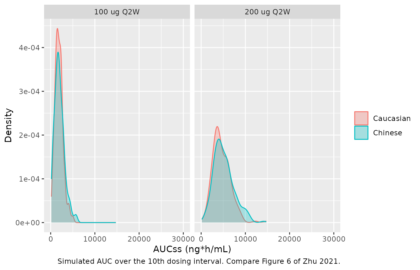


fig6 <- auc_ss |>
  dplyr::group_by(regimen, population) |>
  dplyr::summarise(
    sim_p10 = quantile(PPORRES, 0.1), sim_p50 = median(PPORRES),
    sim_p90 = quantile(PPORRES, 0.9), .groups = "drop"
  ) |>
  dplyr::left_join(
    tibble::tribble(
      ~regimen,       ~population,  ~pub_p10, ~pub_p90,
      "100 ug Q2W",   "Caucasian",      1867,    11595,
      "100 ug Q2W",   "Chinese",        2231,    13403,
      "200 ug Q2W",   "Caucasian",      3776,    14890,
      "200 ug Q2W",   "Chinese",        4384,    16922
    ),
    by = c("regimen", "population")
  )
fig6 |>
  dplyr::rename(
    "Regimen" = regimen, "Population" = population,
    "Simulated P10" = sim_p10, "Simulated median" = sim_p50, "Simulated P90" = sim_p90,
    "Published P10" = pub_p10, "Published P90" = pub_p90
  ) |>
  knitr::kable(digits = 0, caption = "AUCss 80% intervals (ng*h/mL): simulation vs. Zhu 2021 Results / Figure 6.")

AUCss 80% intervals (ng*h/mL): simulation vs. Zhu 2021 Results / Figure 6.
Regimen	Population	Simulated P10	Simulated median	Simulated P90	Published P10	Published P90
100 ug Q2W	Caucasian	858	1815	3078	1867	11595
100 ug Q2W	Chinese	682	1806	3415	2231	13403
200 ug Q2W	Caucasian	2310	4289	7035	3776	14890
200 ug Q2W	Chinese	2651	4707	8186	4384	16922


stopifnot(
  # The paper's qualitative conclusion: Chinese exposure is similar to, and
  # slightly higher than, Caucasian exposure at the same dose (lower weight,
  # so lower CL/F). Compare medians, which are robust to the cohort draw.
  all(with(fig6, sim_p50[population == "Chinese"] / sim_p50[population == "Caucasian"]) > 0.8),
  all(with(fig6, sim_p50[population == "Chinese"] / sim_p50[population == "Caucasian"]) < 1.5)
)

# Upper bound from the linear arm alone: with no target-mediated
# elimination, AUC over one interval at steady state is exactly
# Dose / (CL/F), so its 90th percentile at the mean weight is
# Dose / CL_typ * exp(qnorm(0.9) * omega_CL). The target arm can only
# lower the AUC, so no reading of Table 2 reaches the published P90.
omega_cl <- sqrt(log(0.357^2 + 1))
linear_p90 <- fig6 |>
  dplyr::mutate(
    dose = ifelse(regimen == "100 ug Q2W", 100, 200),
    wt = ifelse(population == "Caucasian", 79.4, 68.1),
    lin_p90 = dose / (0.778 / 24 * (wt / 70)^0.927) * exp(qnorm(0.9) * omega_cl)
  )
linear_p90 |> dplyr::select(regimen, population, lin_p90, pub_p90)
#> # A tibble: 4 × 4
#>   regimen    population lin_p90 pub_p90
#>   <chr>      <chr>        <dbl>   <dbl>
#> 1 100 ug Q2W Caucasian    4278.   11595
#> 2 100 ug Q2W Chinese      4933.   13403
#> 3 200 ug Q2W Caucasian    8557.   14890
#> 4 200 ug Q2W Chinese      9865.   16922
stopifnot(all(linear_p90$lin_p90 < 0.7 * linear_p90$pub_p90))

The simulated 80% intervals are narrower and lower than those printed for Figure 6. The linear part of the model alone bounds the published upper limits: with no target-mediated elimination at all, the steady-state AUC over one interval is exactly Dose / (CL/F), and the 90th percentile of that quantity at 100 ug is about 4,300 ng*h/mL for a 79.4 kg subject and about 4,900 ng*h/mL for a 68.1 kg subject given the 35.7% BSV on CL/F, against the published 11,595 and 13,403 ng*h/mL. The target-mediated arm can only lower the AUC further. The Figure 6 intervals therefore cannot be reproduced from Table 2 by any reading of its units; the Simulx settings used for Figure 6 are not reported, so the discrepancy is recorded rather than resolved. The single-dose NCA comparison above, which is the paper’s direct data summary, is reproduced.

Assumptions and deviations

Mixed printed time units. Table 2 and Supplementary Table 2 give CL/F in L/day and ka in 1/day, but tlag, kint and kdeg in hours. The model runs in hours; CL/F and ka are divided by 24 in ini(). The per-hour reading of kint and kdeg is the one the paper’s own single-dose NCA supports (see the unit check above). tlag is 0.426 h either way in effect: observed profiles are quantifiable at the 1 h sample.
Observed quantity. The paper defines both Ctotal and Cfree (Equations 3-6) but does not state which one the observations were fitted to. The model reports total drug, Cc = central / vc, the conventional choice for a quasi-equilibrium TMDD model fitted to a sandwich immunoassay; above about 1 ng/mL the two differ by at most the receptor pool (well under 1 ng/mL).
Between-subject variability scale. Table 2 reports BSV as CV% without stating the conversion. The variances are omega^2 = log(CV^2 + 1), the exact log-normal relation; with the approximation omega^2 = CV^2 the V/F variance would be 0.82 instead of 0.60.
Residual error. Equation 12, Y = IPRED * (1 + eps_prop) + eps_add, with the two epsilons reported separately, is encoded as the nlmixr2 combined additive + proportional error; the 18.7% and 0.342 ng/mL are taken as standard deviations, as the Table 2 units indicate.
Weight reference. Equation 15 divides weight by 70 kg, and the abstract and Discussion quote CL/F “in 70-kg subjects”; the Methods text calls the reference “the median value”, which is not reported. 70 kg is used as printed.
Virtual cohort. Weights are normal with the Table 1 mean and SD for each study; sex is not needed because it is not in the model. The simulation applies no quantification-limit censoring.
Figure 6. The published steady-state 80% intervals are not reproduced (see above).