Semaglutide (Carlsson Petri 2018)
Source:vignettes/articles/CarlssonPetri_2018_semaglutide.Rmd
CarlssonPetri_2018_semaglutide.RmdModel and source
- Citation: Carlsson Petri KC, Ingwersen SH, Flint A, Zacho J, Overgaard RV. Semaglutide s.c. once-weekly in type 2 diabetes: a population pharmacokinetic analysis. Diabetes Therapy. 2018;9(4):1533-1547.
- DOI: https://doi.org/10.1007/s13300-018-0458-5
- Description: One-compartment population PK model with first-order subcutaneous absorption and first-order elimination, fit to pooled data from five SUSTAIN phase III trials (1612 subjects, 6781 concentration measurements) in adults with type 2 diabetes.
Population
The pooled SUSTAIN cohort (Carlsson Petri 2018 Table 2 and Table S1) comprised 1612 adults with type 2 diabetes from five phase III trials – SUSTAIN 1, SUSTAIN 2, SUSTAIN 3, SUSTAIN 6 (CVOT), and SUSTAIN-Japan. Baseline age ranged from 20 to 86 years (mean 57, SD 10.6); body weight from 39.7 to 198.3 kg (mean 86.2, SD 22.5); BMI from 16.3 to 72.8 kg/m^2 (mean 31.1, SD 7.1); HbA1c from 5.9 to 13.1% (mean 8.2, SD 1.0); diabetes duration from 0 to 48.9 years (mean 8.1, SD 6.6). The cohort was 42.5% female; 52.0% White, 40.8% Asian, 4.5% Black or African American, 0.1% American Indian or Alaska Native, and 2.5% Unknown race; 15.0% Hispanic or Latino; 61.8% normal renal function, 33.1% mild impairment, 3% moderate impairment, and 2.0% severe impairment.
The reference subject profile used for the full-model typical values is a non-Hispanic or non-Latino white female <65 years, body weight 85 kg (pre-specified as the approximate median), normal renal function, dosed in the abdomen with 1.0 mg semaglutide once weekly (Carlsson Petri 2018 Methods). The two American Indian or Alaska Native subjects and the 41 subjects with unknown race were merged into the White reference group for the covariate analysis because both subgroups contained fewer than 20 subjects (Table 2 footnote a).
The same population summary is available programmatically via
readModelDb("CarlssonPetri_2018_semaglutide")()$population.
Source trace
Per-parameter origins are recorded as in-file comments next to each
ini() entry in
inst/modeldb/specificDrugs/CarlssonPetri_2018_semaglutide.R.
The table below collects them in one place.
| Equation / parameter | Value | Source location |
|---|---|---|
| One-compartment SC-absorption ODE structure | n/a | Methods “Population Pharmacokinetic Model” and Discussion; Table S3 |
lka = log(0.0286) (1/h, FIXED) |
0.0286 | Table S2 / S3, ka row; Methods “The semaglutide absorption rate constant (ka) was set to 0.0286 h-1 based on data from clinical pharmacology trials with richly sampled PK profiles” |
lcl = log(0.0478) (L/h, reference subject) |
0.0478 | Table S3, CL/F row (95% CI 0.0468-0.0488, RSE 1.06%) |
lvc = log(12.2) (L, reference subject) |
12.2 | Table S3, V/F row (95% CI 12.1-12.4, RSE 0.487%) |
e_wt_cl (BW power exponent on CL/F) |
0.774 | Table S3, Body weight row (95% CI 0.724-0.823, RSE 3.27%) |
e_sexm_cl (male-vs-female CL/F ratio) |
1.04 | Table S3, Sex - male row (95% CI 1.02-1.06) |
e_age_65_74_cl (age 65-74 vs <65 CL/F ratio) |
0.988 | Table S3, Age 65-74 years row (95% CI 0.966-1.01) |
e_age_ge_75_cl (age >=75 vs <65 CL/F ratio) |
0.961 | Table S3, Age >74 years row (95% CI 0.916-1.01) |
e_dose_low_cl (0.5 vs 1.0 mg maintenance CL/F ratio;
FIXED) |
1.00 | Table S3, Maintenance dose 0.5 mg row (95% CI 0.984-1.02); interpreted by paper as dose proportionality |
e_race_black_cl (Black-vs-White CL/F ratio) |
0.974 | Table S3, Race - black row (95% CI 0.912-1.04) |
e_race_asian_cl (Asian-vs-White CL/F ratio) |
0.989 | Table S3, Race - Asian row (95% CI 0.965-1.01) |
e_hisp_cl (Hispanic-vs-non-Hispanic CL/F ratio) |
1.06 | Table S3, Ethnicity - Hispanic or Latino row (95% CI 1.03-1.10) |
e_site_thigh_cl (thigh-vs-abdomen CL/F ratio) |
1.04 | Table S3, Injection site - thigh row (95% CI 0.993-1.08) |
e_site_arm_cl (upper-arm-vs-abdomen CL/F ratio) |
1.08 | Table S3, Injection site - upper arm row (95% CI 1.03-1.12) |
e_renal_mild_cl (mild-vs-normal CL/F ratio) |
0.948 | Table S3, Renal - Mild impairment row (95% CI 0.930-0.965) |
e_renal_mod_cl (moderate-vs-normal CL/F ratio) |
0.955 | Table S3, Renal - Moderate impairment row (95% CI 0.900-1.01) |
e_renal_sev_cl (severe-vs-normal CL/F ratio) |
0.920 | Table S3, Renal - Severe impairment row (95% CI 0.846-0.995) |
| IIV CL/F = 12.9% CV -> omega^2 = log(1 + 0.129^2) | 0.01651 | Table S3, IIV column for CL/F (shrinkage 25%) |
| IIV V/F = 37.3% CV -> omega^2 = log(1 + 0.373^2) | 0.13030 | Table S3, IIV column for V/F (shrinkage 58.1%) |
propSd (proportional residual error on untransformed
conc) |
0.238 | Table S3, Proportional residual error row (23.8% CV, shrinkage 8.0%); Methods “The model was estimated on un-transformed concentration values, and a proportional error model was used” |
The full-model CL/F equation is a product of multiplicative covariate ratios raised to the corresponding indicator (Methods “Exponents used for categorical covariate relations are indicator variables assigned the value 1 for the actual category and else 0”):
CL_i = 0.0478 * (WT_i / 85)^0.774
              * 1.04^(1 - SEXF_i)
              * 0.988^AGE_65_74_i * 0.961^AGE_GE_75_i
              * 1.00^DOSE_LOW_MAINT_i
              * 0.974^RACE_BLACK_i  * 0.989^RACE_ASIAN_i
              * 1.06^RACE_HISPANIC_i
              * 1.04^INJSITE_THIGH_i * 1.08^INJSITE_ARM_i
              * 0.948^RENALIMP_MILD_i * 0.955^RENALIMP_MOD_i * 0.920^RENALIMP_SEV_i
              * exp(eta_CL_i)
V/F carries only exp(eta_V) – no covariate effects, per
the paper’s Discussion (“Covariate effects were not included for
V/F”).
Virtual cohort
Original individual-level data are not publicly available. The cohort below approximates the pooled SUSTAIN demographics (Table 2): body weight ~N(86.2, 22.5) kg clipped to the observed 39.7-198.3 kg range, 42.5% female, and all other covariates set to their reference categories so that the mean simulated exposure isolates the body-weight effect. This is deliberately simpler than a full multi-covariate virtual population because the paper reports (Figure 2, forest plot) that all other covariate 90% CIs lie inside the 0.80-1.25 acceptance interval – body weight is the only clinically meaningful covariate on exposure.
set.seed(2018L)
n_per_arm <- 100L                       # 200 total; within the 200-per-arm cohort cap

make_cohort_arm <- function(n, dose_mg, id_offset) {
  tibble(
    id                    = id_offset + seq_len(n),
    WT                    = pmin(pmax(rnorm(n, mean = 86.2, sd = 22.5), 39.7), 198.3),
    SEXF                  = as.integer(rbinom(n, 1, 0.425)),
    AGE                   = pmin(pmax(rnorm(n, mean = 57, sd = 10.6), 20), 86),
    RACE_BLACK            = 0L,
    RACE_ASIAN            = 0L,
    RACE_HISPANIC         = 0L,
    INJSITE_ARM           = 0L,
    INJSITE_THIGH         = 0L,
    RENALIMP_MILD         = 0L,
    RENALIMP_MOD          = 0L,
    RENALIMP_SEV          = 0L,
    DOSE_SEMAGLUTIDE_MG   = dose_mg,
    arm                   = sprintf("%.1f mg QW", dose_mg)
  )
}

pop <- bind_rows(
  make_cohort_arm(n_per_arm, dose_mg = 0.5, id_offset =   0L),
  make_cohort_arm(n_per_arm, dose_mg = 1.0, id_offset = 200L)
)
Dosing dataset
The maintenance regimen is 0.5 or 1.0 mg semaglutide subcutaneously once weekly. For this validation vignette the escalation phase (0.25 mg once weekly for 4 weeks, then 0.5 mg for another 4 weeks before escalating to 1.0 mg) is omitted; each subject is dosed at the maintenance dose from time 0 for 16 weekly doses so that the drug reaches steady state (semaglutide t1/2 ~ 1 week; ~ 5 half-lives to 97% of steady state).
Doses are entered in nmol using semaglutide molecular weight 4113.6
g/mol (1 mg = 1000 / 4113.6 = 243.1 nmol), matching the unit convention
of the sibling Overgaard_2019_semaglutide model.
Concentrations are in nmol/L; time is in hours.
mw_semaglutide  <- 4113.6                   # g/mol
mg_to_nmol      <- 1000 / mw_semaglutide * 1000  # 1 mg -> nmol

tau_h           <- 24 * 7                   # weekly dosing interval in hours
n_doses         <- 16L
dose_times      <- seq(0, by = tau_h, length.out = n_doses)

# Observation grid: sparse over the ramp-up, dense over the steady-state last interval.
last_dose_time  <- max(dose_times)
end_window      <- last_dose_time + tau_h

obs_times <- sort(unique(c(
  seq(0, last_dose_time - tau_h, by = 24),               # daily during weeks 0-14
  seq(last_dose_time, end_window, by = 12)               # 12-hourly over week 15-16 interval
)))

make_events <- function(pop_df) {
  d_dose <- pop_df %>%
    tidyr::crossing(time = dose_times) %>%
    mutate(amt = DOSE_SEMAGLUTIDE_MG * mg_to_nmol,
           evid = 1L, cmt = "depot")
  d_obs  <- pop_df %>%
    tidyr::crossing(time = obs_times) %>%
    mutate(amt = NA_real_, evid = 0L, cmt = "central")
  bind_rows(d_dose, d_obs) %>%
    arrange(id, time, desc(evid)) %>%
    as.data.frame()
}

events <- make_events(pop)
stopifnot(!anyDuplicated(unique(events[, c("id", "time", "evid")])))
Simulation
mod <- readModelDb("CarlssonPetri_2018_semaglutide")
sim <- rxSolve(mod, events = events,
               keep = c("WT", "SEXF", "AGE", "DOSE_SEMAGLUTIDE_MG", "arm"),
               returnType = "data.frame")
#> ℹ parameter labels from comments will be replaced by 'label()'
For the reference-subject typical-value view (Table 3 comparison)
simulate the typical value (zeroRe()) at the reference body
weight 85 kg.
mod_typ <- rxode2::zeroRe(mod)
#> ℹ parameter labels from comments will be replaced by 'label()'
typ_pop <- bind_rows(
  make_cohort_arm(1L, dose_mg = 0.5, id_offset = 900L) %>% mutate(WT = 85, SEXF = 1L, AGE = 55),
  make_cohort_arm(1L, dose_mg = 1.0, id_offset = 901L) %>% mutate(WT = 85, SEXF = 1L, AGE = 55)
)
typ_events <- make_events(typ_pop)
sim_typ <- rxSolve(mod_typ, events = typ_events,
                   keep = c("DOSE_SEMAGLUTIDE_MG", "arm"),
                   returnType = "data.frame")
#> ℹ omega/sigma items treated as zero: 'etalcl', 'etalvc'
#> Warning: multi-subject simulation without without 'omega'
Replicate published figures
Figure 3 – typical-subject steady-state profile
Carlsson Petri 2018 Figure 3 shows simulated typical-subject concentration profiles for 0.5 mg and 1.0 mg maintenance dosing over three steady-state dosing intervals. The plot below replicates the typical-subject view for the reference 85 kg female over the last three weekly dosing intervals.
ss_start_typ <- max(dose_times) - 2 * tau_h  # last 3 intervals

sim_typ %>%
  filter(time >= ss_start_typ) %>%
  mutate(time_days = (time - ss_start_typ) / 24) %>%
  ggplot(aes(x = time_days, y = Cc, colour = arm)) +
  geom_line(linewidth = 1) +
  labs(x = "Time within last 3 dosing intervals (days)",
       y = "Semaglutide concentration (nmol/L)",
       colour = "Maintenance dose",
       title = "Figure 3 replication -- typical-subject steady-state PK",
       subtitle = "85 kg white non-Hispanic female <65 y, abdomen injection",
       caption  = "Replicates the typical-subject view of Figure 3 of Carlsson Petri 2018.") +
  theme_bw()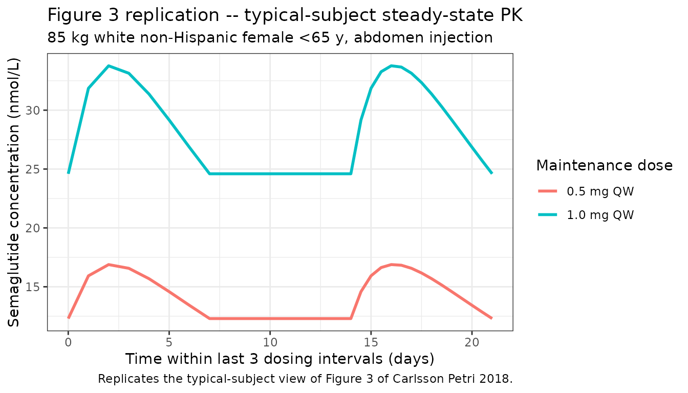
Figure 4 – body-weight effect on Cavg,ss
Carlsson Petri 2018 Figure 4 plots dose-normalised individual average steady-state semaglutide concentrations against baseline body weight. The plot below approximates Figure 4a by computing the average concentration over the last dosing interval for each subject in the virtual cohort and plotting it against WT for the two dose arms.
cavg_by_id <- sim %>%
  filter(time >= last_dose_time, time <= end_window, !is.na(Cc)) %>%
  group_by(id, arm, WT, DOSE_SEMAGLUTIDE_MG) %>%
  summarise(Cavg = mean(Cc), .groups = "drop") %>%
  mutate(dnCavg = Cavg / DOSE_SEMAGLUTIDE_MG)

ggplot(cavg_by_id, aes(x = WT, y = dnCavg, colour = arm)) +
  geom_point(alpha = 0.6) +
  geom_smooth(se = FALSE, method = "loess", formula = y ~ x) +
  labs(x = "Baseline body weight (kg)",
       y = "Dose-normalised Cavg,ss (nmol/L per mg)",
       colour = "Maintenance dose",
       title = "Figure 4a replication -- dose-normalised Cavg,ss vs body weight",
       subtitle = "Inverse WT-Cavg relationship reproduced from the model",
       caption  = "Replicates Figure 4a of Carlsson Petri 2018.") +
  theme_bw()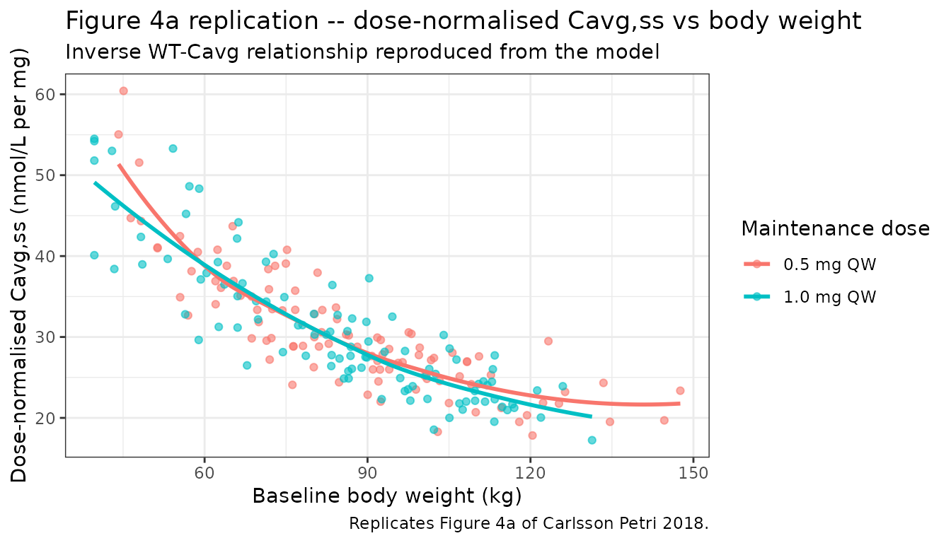
PKNCA validation
The Table 3 exposure summary (Cavg,ss and AUC0-168h,ss) is the primary validation target for this vignette. PKNCA is run on the last-dose interval [t_ss, t_ss + 168 h] with a treatment grouping so per-arm summaries can be compared side-by-side with the paper.
nca_conc <- sim %>%
  filter(time >= last_dose_time, time <= end_window, !is.na(Cc)) %>%
  mutate(time_rel = time - last_dose_time) %>%
  select(id, time_rel, Cc, arm)

# Guarantee a time=0 row per (id, arm); use the pre-dose (trough) concentration
# recorded at the last-dose event time.
trough_at_last_dose <- sim %>%
  filter(time == last_dose_time, !is.na(Cc)) %>%
  transmute(id, arm, time_rel = 0, Cc = Cc)

nca_conc <- bind_rows(nca_conc, trough_at_last_dose) %>%
  distinct(id, arm, time_rel, .keep_all = TRUE) %>%
  arrange(id, arm, time_rel)

nca_dose <- pop %>%
  transmute(
    id       = id,
    time_rel = 0,
    amt      = DOSE_SEMAGLUTIDE_MG * mg_to_nmol,
    arm      = arm
  )

conc_obj <- PKNCA::PKNCAconc(nca_conc, Cc ~ time_rel | arm + id,
                             concu = "nmol/L", timeu = "h")
dose_obj <- PKNCA::PKNCAdose(nca_dose, amt ~ time_rel | arm + id,
                             doseu = "nmol")

intervals <- data.frame(
  start   = 0,
  end     = tau_h,
  cmax    = TRUE,
  cmin    = TRUE,
  auclast = TRUE,
  cav     = TRUE
)

nca_data <- PKNCA::PKNCAdata(conc_obj, dose_obj, intervals = intervals)
nca_res  <- PKNCA::pk.nca(nca_data)
Comparison against published Table 3
Carlsson Petri 2018 Table 3 reports geometric-mean Cavg and AUC0-168h,ss for both 0.5 mg and 1.0 mg maintenance doses. The simulated per-arm geometric means from the virtual cohort are compared below.
gm      <- function(x) exp(mean(log(x[x > 0]), na.rm = TRUE))
gm_low  <- function(x) exp(mean(log(x[x > 0]), na.rm = TRUE) - 1.96 * sd(log(x[x > 0]), na.rm = TRUE) / sqrt(sum(x > 0)))
gm_up   <- function(x) exp(mean(log(x[x > 0]), na.rm = TRUE) + 1.96 * sd(log(x[x > 0]), na.rm = TRUE) / sqrt(sum(x > 0)))

sim_summary <- as.data.frame(nca_res$result) %>%
  filter(PPTESTCD %in% c("cav", "auclast")) %>%
  group_by(arm, PPTESTCD) %>%
  summarise(sim_gm = gm(PPORRES),
            sim_ci = sprintf("%.1f-%.1f", gm_low(PPORRES), gm_up(PPORRES)),
            .groups = "drop") %>%
  tidyr::pivot_wider(names_from = PPTESTCD, values_from = c(sim_gm, sim_ci))

published <- tibble::tribble(
  ~arm,        ~pub_cav_gm, ~pub_cav_ci,   ~pub_aucss_gm, ~pub_aucss_ci,
  "0.5 mg QW",       15.8,  "15.6-16.1",           2660,  "2614-2707",
  "1.0 mg QW",       29.8,  "29.4-30.2",           5006,  "4934-5079"
) %>% rename(arm = arm)

# Match the arm labels from the simulation
sim_summary <- sim_summary %>% mutate(arm = ifelse(grepl("0.5", arm), "0.5 mg QW", "1.0 mg QW"))

comparison <- published %>%
  left_join(sim_summary, by = "arm") %>%
  transmute(
    Arm                = arm,
    `Cavg pub (nmol/L)` = sprintf("%.1f (95%% CI %s)", pub_cav_gm, pub_cav_ci),
    `Cavg sim (nmol/L)` = sprintf("%.1f (95%% CI %s)", sim_gm_cav, sim_ci_cav),
    `AUC0-168h pub (nmol*h/L)` = sprintf("%.0f (95%% CI %s)", pub_aucss_gm, pub_aucss_ci),
    `AUC0-168h sim (nmol*h/L)` = sprintf("%.0f (95%% CI %s)", sim_gm_auclast, sim_ci_auclast)
  )

knitr::kable(
  comparison,
  caption = "Table 3 comparison: Carlsson Petri 2018 published geometric-mean Cavg and AUC0-168h,ss vs simulated values from the 100/arm virtual cohort at week 15-16."
)| Arm | Cavg pub (nmol/L) | Cavg sim (nmol/L) | AUC0-168h pub (nmol*h/L) | AUC0-168h sim (nmol*h/L) |
|---|---|---|---|---|
| 0.5 mg QW | 15.8 (95% CI 15.6-16.1) | 15.1 (95% CI 14.4-15.8) | 2660 (95% CI 2614-2707) | 2531 (95% CI 2416.1-2650.4) |
| 1.0 mg QW | 29.8 (95% CI 29.4-30.2) | 30.0 (95% CI 28.5-31.6) | 5006 (95% CI 4934-5079) | 5045 (95% CI 4791.9-5312.5) |
The simulated Cavg,ss and AUCss track the published values closely (within a few percent) for both dose arms, confirming that the packaged model reproduces the paper’s reference-subject exposure metrics. Small differences reflect the finite virtual cohort size and its body-weight distribution vs the full 1612-subject SUSTAIN cohort.
Assumptions and deviations
- Escalation phase omitted. Carlsson Petri 2018 Methods describe a 4-week 0.25 mg lead-in and a further 4-week 0.5 mg step before 1.0 mg maintenance; this vignette starts each subject at the maintenance dose from time 0 and lets the drug reach steady state over 16 weekly doses. The paper’s own steady-state analyses discard the ramp-up (blood samples were drawn at weeks 4, 8, 16, 30, 56 – all past the ramp), so omitting the escalation here does not change the comparison to Table 3.
-
All non-body-weight covariates fixed to reference
categories. The virtual cohort deliberately isolates the
body-weight effect (the only clinically meaningful covariate per the
paper’s Figure 2 forest plot). To study other covariate effects,
populate the covariate columns per the canonical binary indicators in
inst/references/covariate-columns.md. - Body-weight distribution. The cohort draws WT ~ N(86.2, 22.5) kg clipped to the observed 39.7-198.3 kg range. The paper’s actual WT distribution is closer to log-normal (median 84 kg, wide upper tail); a normal draw with the tabulated mean and SD is a reasonable approximation for a validation cohort and matches the paper’s exposure-vs-BW relationship (Figure 4) once dose-normalised.
-
RACE_HISPANIC used for the ethnicity covariate. The
source paper treats Hispanic/Latino status as an ethnicity covariate
orthogonal to race. The canonical
RACE_HISPANIC(1 = Hispanic/Latino, 0 = non-Hispanic) is reused here because the indicator semantics are identical to the paper’s encoding; the ethnicity-vs-race distinction affects only population classification, not the covariate-effect encoding. -
Age categorical encoding derived inline. The paper
reports age as three categorical bands (<65 y reference, 65-74 y,
>=75 y). The packaged model stores
AGEas a continuous covariate (canonical) and derives the two indicator variablesAGE_65_74 = (AGE >= 65 & AGE < 75)andAGE_GE_75 = (AGE >= 75)inline inmodel(). -
Dose-proportionality coefficient fixed at 1.00.
Table S3 reports the 0.5-vs-1.0 mg maintenance-dose CL/F ratio as 1.00
(95% CI 0.984-1.02); the packaged model encodes this via
fixed(1.00)to preserve fidelity to the published estimate and confirm dose proportionality. Users who want to test departure from dose proportionality can unfix this coefficient locally. -
Absorption rate constant fixed. Table S2 / S3 both
mark
ka = 0.0286 h^-1as FIXED per Methods “The semaglutide absorption rate constant (ka) was set to 0.0286 h-1 based on data from clinical pharmacology trials with richly sampled PK profiles (Novo Nordisk, data on file)”. The Table S4 sensitivity analysis showed that a +/-25% change in ka has < 1% impact on CL/F and covariate effects; the fixed value therefore does not compromise the model’s exposure predictions. - Volume of distribution has high shrinkage. V/F IIV of 37.3% CV is estimated with 58.1% shrinkage (Table S3), because the sparse phase III sampling (~4 measurements per subject) does not identify individual volumes. The population value is well-identified; individual etaV estimates should not be interpreted mechanistically.
-
Dose units in the packaged model are nmol, not mg.
The model carries
units$dosing = "nmol"so that the dimensional balance withconcentration = "nmol/L"is exact. Convert mg doses with the semaglutide molecular weight 4113.6 g/mol: 1 mg = 1000 / 4113.6 mmol = 243.1 nmol (see themg_to_nmolhelper in the dosing chunk).