Perioperative factor VIII after Haemate P in von Willebrand disease (de Jager 2020)
Source:vignettes/articles/deJager_2020_factorviii.Rmd
deJager_2020_factorviii.RmdModel and source
- Citation: de Jager NCB, Bukkems LH, Heijdra JM, Hazendonk HCAM, Fijnvandraat K, Meijer K, Eikenboom J, Laros-van Gorkom BAP, Leebeek FWG, Cnossen MH, Mathot RAA; OPTI-CLOT group. One piece of the puzzle: Population pharmacokinetics of FVIII during perioperative Haemate P/Humate P treatment in von Willebrand disease patients. J Thromb Haemost. 2020;18(2):295-305.
- Article: https://doi.org/10.1111/jth.14652 (open access, PMC7028136)
- Supplement: Appendix S1 (population PK equations and validation goodness-of-fit plots), on the article page.
- Description: one-compartment population PK model for factor VIII (FVIII) activity after the plasma-derived VWF/FVIII concentrate Haemate P / Humate P (VWF:FVIII ratio 2.4:1), given perioperatively to patients with von Willebrand disease (VWD). The model is built on FVIII levels only; VWF activity enters as a time-varying covariate on FVIII clearance.
The final model (Table 2 footnote and Appendix S1 Eq. 2-5) is
with V in L, CL in L/h and FVIII in IU/mL. The baseline is the lowest FVIII ever measured in the patient.
The paper also fits a virtual dose. In 92 of 180
surgeries the FVIII level measured before the first concentrate dose was
higher than the patient’s lowest-ever baseline. The authors gave these
patients a fixed virtual dose before the pre-dose sample, with an
estimated bioavailability (F = 0.200, inter-occasion variability 154.5%
CV). The virtual dose carries the endogenous FVIII above baseline, which
then decays back to the lowest-ever level. The packaged model gives this
dose its own state, virtual, which eliminates at the same
rate as central and has f(virtual) set to the
fitted F. Real doses go to central with F = 1. The paper
does not report the virtual dose amount, because only the product of
amount and F is identifiable.
Population
The final model was estimated on all available data (Table 1): 117 patients with VWD who underwent 172 surgeries at five Dutch academic haemophilia treatment centres between 2000 and 2018. These data were 97 patients (141 surgeries, 684 FVIII samples) in the index set and 20 patients (31 surgeries, 208 samples) in the external-validation set. Median age was 50 years (0.5-82; seven children), median weight 77.0 kg (8.8-118.0), and 67% were female. VWD type per occasion was 1 (47%), 2A (27%), 2B (6%), 2M (11%), 2N (5%) and 3 (5%). ASA class was II for 83% of occasions, III for 16% and IV for 1%. 72% of surgeries were major. Median surgery duration was 65 min (7-470). Patients received a median of 5 Haemate P doses per occasion, at a median 20.8 IU FVIII/kg (5.5-66.1). Median lowest-ever FVIII was 0.41 IU/mL (0.01-0.97).
The same information is available programmatically via
readModelDb("deJager_2020_factorviii")()$population.
Source trace
| Equation / parameter | Value | Source location |
|---|---|---|
lvc |
log(3.28 L) at 70 kg | Table 2, Final FVIII Estimate, Volume of distribution |
lcl |
log(0.037 L/h) at 70 kg | Table 2, Final, Clearance |
lfvirtual |
log(0.200) | Table 2, Final, Bioavailability virtual dose; Appendix S1 Eq. 3 |
e_wt_vc |
1 (fixed a priori) | Methods 2.2; Appendix S1 Eq. 4; Table 2 footnote |
e_wt_cl |
0.75 (fixed a priori) | Methods 2.2; Appendix S1 Eq. 5; Table 2 footnote |
e_tsurg_cl |
-0.416, reference 81 min | Table 2, Final, Surgery duration on CL; footnote |
e_asa_ge3_cl |
0.555 | Table 2, Final, ASA class III or IV on CL; footnote |
e_vwf_cl |
-0.263, reference 1.65 IU/mL | Table 2, Final, VWF activity on CL; footnote |
etalcl, etalvc
|
84.1% CV, 30.9% CV, r = 0.47 | Table 2, Final, IIV CL, IIV V, correlation; CV definition in Table 2 abbreviations |
etaiov_lfvirtual_1 |
154.5% CV | Table 2, Final, IOV bioavailability virtual dose |
propSd |
0.203 | Table 2, Final, proportional residual variability; Appendix S1 Eq. 2 |
| one-compartment IV structure | n/a | Results 3.1 |
observation
Cc = (central + virtual)/vc/1000 + FVIII_BL
|
n/a | Appendix S1 Eq. 2; Methods 2.2 |
| virtual dose | n/a | Methods 2.2; Results 3.1 |
Variances are omega^2 = log(1 + CV^2), following the CV
definition in the Table 2 abbreviations. The V-CL covariance is
0.47 * sqrt(omega^2_CL * omega^2_V).
Typical-value checks against the paper’s numbers
mod <- readModelDb("deJager_2020_factorviii")

# Table 2 footnote, with surgery duration in minutes and VWF:Act in IU/mL.
typ_cl <- function(wt, dur_min, vwf_iu_ml, asa34) {
  0.037 * (wt / 70)^0.75 * (dur_min / 81)^-0.416 * (vwf_iu_ml / 1.65)^-0.263 * 0.555^asa34
}
typ_v <- function(wt) 3.28 * (wt / 70)

chk_cov <- data.frame(
  id = 1:5,
  WT = c(70, 70, 50, 90, 25),
  dur_min = c(81, 45, 106, 240, 30),
  vwf_iu_ml = c(1.65, 0.78, 2.21, 3.0, 0.5),
  ASA_GE3 = c(0, 0, 1, 1, 0),
  FVIII_BL = 0
) |>
  mutate(T_SURG = dur_min / 60, VWF = vwf_iu_ml * 100)
ev_chk <- bind_rows(
  chk_cov |> mutate(time = 0, evid = 1L, amt = 1000, cmt = "central"),
  chk_cov |> mutate(time = 1, evid = 0L, amt = 0, cmt = "central")
) |>
  arrange(id, time, desc(evid)) |>
  as.data.frame()
sim_chk <- as.data.frame(rxSolve(zeroRe(mod), ev_chk, keep = c("WT", "dur_min", "vwf_iu_ml", "ASA_GE3")))
#> ℹ parameter labels from comments will be replaced by 'label()'
#> ℹ omega/sigma items treated as zero: 'etalcl', 'etalvc', 'etaiov_lfvirtual_1'
#> Warning: multi-subject simulation without without 'omega'
sim_chk <- sim_chk[!duplicated(sim_chk$id), ]

# Same parameters on both sides, so the packaged model must match the
# footnote to floating-point precision.
stopifnot(
  all(abs(sim_chk$cl / typ_cl(sim_chk$WT, sim_chk$dur_min, sim_chk$vwf_iu_ml, sim_chk$ASA_GE3) - 1) < 1e-10),
  all(abs(sim_chk$vc / typ_v(sim_chk$WT) - 1) < 1e-10)
)

ref_t12 <- log(2) * typ_v(70) / typ_cl(70, 81, 1.65, 0)
tibble::tibble(
  Quantity = c(
    "Typical t1/2 at 70 kg, 81 min, VWF:Act 1.65 IU/mL, ASA II (h)",
    "CL change, surgery duration 45 -> 106 min (%)",
    "CL change, VWF:Act 0.78 -> 2.21 IU/mL (%)",
    "CL change, ASA III/IV vs II (%)"
  ),
  `From packaged model` = round(c(
    ref_t12,
    100 * ((106 / 45)^-0.416 - 1),
    100 * ((2.21 / 0.78)^-0.263 - 1),
    100 * (0.555 - 1)
  ), 1),
  Paper = c(
    "57.7 (median individual t1/2, Discussion)",
    "-38 (Results 3.2)",
    "-29 (Results 3.2)",
    "-44 (Results 3.2)"
  )
) |>
knitr::kable(caption = "Typical values from the packaged model versus the numbers quoted in de Jager 2020.")| Quantity | From packaged model | Paper |
|---|---|---|
| Typical t1/2 at 70 kg, 81 min, VWF:Act 1.65 IU/mL, ASA II (h) | 61.4 | 57.7 (median individual t1/2, Discussion) |
| CL change, surgery duration 45 -> 106 min (%) | -30.0 | -38 (Results 3.2) |
| CL change, VWF:Act 0.78 -> 2.21 IU/mL (%) | -24.0 | -29 (Results 3.2) |
| CL change, ASA III/IV vs II (%) | -44.5 | -44 (Results 3.2) |
The ASA effect agrees with the text. The two interquartile-range contrasts quoted in Results 3.2 are larger than the printed exponents give: 38% versus 30% for surgery duration, and 29% versus 24% for VWF activity. No exponent printed in Table 2 (structural, intermediate, final or bootstrap) reproduces the text: the intermediate-model exponents give 31% and 27%. The Table 2 equation is used, and the difference is noted under Assumptions and deviations. The typical half-life of 61 h at the reference covariates sits close to the paper’s 57.7 h median individual half-life. The PKNCA section below checks the cohort median.
Replicate Figure 1: clearance versus VWF activity and surgery duration
grid_vwf <- data.frame(vwf_iu_ml = exp(seq(log(0.1), log(5), length.out = 60)), dur_min = 81, panel = "A: VWF activity")
grid_dur <- data.frame(vwf_iu_ml = 1.65, dur_min = exp(seq(log(7), log(470), length.out = 60)), panel = "B: surgery duration")
fig1 <- bind_rows(grid_vwf, grid_dur) |>
  mutate(
    id = row_number(), WT = 70, ASA_GE3 = 0, FVIII_BL = 0,
    T_SURG = dur_min / 60, VWF = vwf_iu_ml * 100,
    x = ifelse(panel == "A: VWF activity", vwf_iu_ml, dur_min)
  )
ev_fig1 <- fig1 |>
  mutate(time = 0, evid = 0L, amt = 0, cmt = "central") |>
  as.data.frame()
sim_fig1 <- as.data.frame(rxSolve(zeroRe(mod), ev_fig1, keep = c("panel", "x")))
#> ℹ parameter labels from comments will be replaced by 'label()'
#> ℹ omega/sigma items treated as zero: 'etalcl', 'etalvc', 'etaiov_lfvirtual_1'
#> Warning: multi-subject simulation without without 'omega'

ggplot(sim_fig1, aes(x, cl)) +
  geom_line() +
  facet_wrap(~panel, scales = "free_x") +
  scale_x_log10() +
  labs(
    x = "VWF:Act (IU/mL) or surgery duration (min)", y = "Typical CL (L/h, 70 kg, ASA II)",
    caption = "Replicates Figure 1A-B of de Jager 2020 (typical clearance curves)."
  ) +
  theme_bw()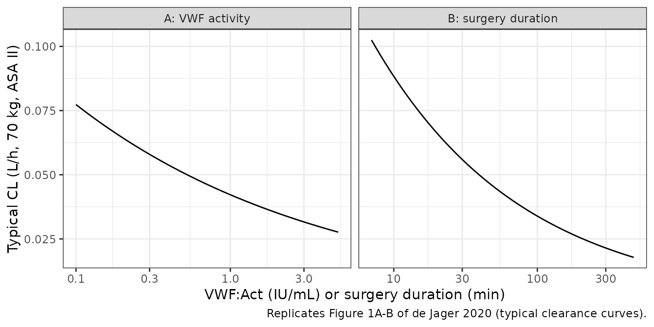
Virtual cohort
Observed data are not public. A virtual cohort of 200 adult-weight surgical occasions follows Table 1. Weight is log-normal around 77 kg, truncated to 40-118 kg. Surgery duration is log-normal around 65 min, truncated to 7-470 min. The lowest-ever FVIII is log-normal around 0.41 IU/mL, truncated to 0.01-0.97 IU/mL. ASA III/IV is assigned with probability 26/152, and VWF:Act is log-normal around the 1.65 IU/mL reference. The spread of VWF:Act is set from the 0.78-2.21 IU/mL interquartile range of measured levels. VWF:Act is held constant within each occasion (see Assumptions and deviations).
set.seed(2020)
rxode2::rxSetSeed(2020)
n_sub <- 200L
tnorm <- function(n, med, sdlog, lo, hi) pmin(pmax(exp(rnorm(n, log(med), sdlog)), lo), hi)

cohort <- tibble::tibble(
  id = seq_len(n_sub),
  WT = tnorm(n_sub, 77, 0.2, 40, 118),
  dur_min = tnorm(n_sub, 65, 0.8, 7, 470),
  VWF = 100 * tnorm(n_sub, 1.65, log(2.21 / 0.78) / (2 * qnorm(0.75)), 0.2, 6),
  ASA_GE3 = as.integer(runif(n_sub) < 26 / 152),
  FVIII_BL = tnorm(n_sub, 0.41, 0.6, 0.01, 0.97),
  treatment = "20.8 IU/kg"
) |>
  mutate(T_SURG = dur_min / 60)

cohort |>
  summarise(
    n = n(),
    `median weight (kg)` = round(median(WT), 1),
    `median surgery duration (min)` = round(median(dur_min)),
    `median VWF:Act (IU/mL)` = round(median(VWF) / 100, 2),
    `ASA III/IV (%)` = round(100 * mean(ASA_GE3)),
    `median baseline FVIII (IU/mL)` = round(median(FVIII_BL), 2)
  ) |>
knitr::kable(caption = "Virtual cohort summary.")| n | median weight (kg) | median surgery duration (min) | median VWF:Act (IU/mL) | ASA III/IV (%) | median baseline FVIII (IU/mL) |
|---|---|---|---|---|---|
| 200 | 78 | 60 | 1.5 | 18 | 0.45 |
Simulation 1: single median dose
A single 20.8 IU/kg dose (the Table 1 median) is given at time 0. The lowest-ever baseline is set to 0 here so the NCA reflects the concentrate alone. The paper’s 57.7 h half-life is computed from the individual PK parameters.
obs_grid <- sort(unique(c(seq(0, 12, 1), seq(14, 72, 2), seq(78, 336, 6))))
ev_single <- bind_rows(
  cohort |> mutate(time = 0, evid = 1L, amt = 20.8 * WT, cmt = "central"),
  cohort |> tidyr::crossing(time = obs_grid) |> mutate(evid = 0L, amt = 0, cmt = "central")
) |>
  mutate(FVIII_BL = 0) |>
  arrange(id, time, desc(evid)) |>
  as.data.frame()

sim_single <- as.data.frame(rxSolve(mod, ev_single, keep = c("treatment", "WT")))
#> ℹ parameter labels from comments will be replaced by 'label()'
PKNCA validation
nca_in <- sim_single |>
  filter(!is.na(Cc)) |>
  select(id, treatment, time, Cc)
nca_in <- bind_rows(
  nca_in,
  nca_in |> distinct(id, treatment) |> mutate(time = 0, Cc = 0)
) |>
  distinct(id, treatment, time, .keep_all = TRUE) |>
  arrange(id, time)

dose_df <- ev_single |>
  filter(evid == 1) |>
  select(id, treatment, time, amt)

conc_obj <- PKNCAconc(nca_in, Cc ~ time | treatment + id, concu = "IU/mL", timeu = "h")
dose_obj <- PKNCAdose(dose_df, amt ~ time | treatment + id, doseu = "IU", route = "intravascular")
intervals <- data.frame(
  start = 0, end = Inf,
  cmax = TRUE, aucinf.obs = TRUE, half.life = TRUE, cl.obs = TRUE
)
nca_res <- pk.nca(PKNCAdata(conc_obj, dose_obj, intervals = intervals))

published <- tibble::tribble(
  ~treatment, ~half.life,
  "20.8 IU/kg", 57.7
)
ncaComparisonTable(
  simulated = nca_res,
  reference = published,
  by = "treatment",
  params = "half.life",
  units = c(half.life = "h"),
  tolerance_pct = 20
) |>
knitr::kable(caption = "Simulated median half-life versus the median individual half-life in de Jager 2020 (Discussion). * differs by more than 20%.")| NCA parameter | treatment | Reference | Simulated | % diff |
|---|---|---|---|---|
| t½ (h) | 20.8 IU/kg | 57.7 | 61.8 | +7.2% |
The NCA half-life must also recover each subject’s own
log(2) * V / CL. The two sides use the same drawn
parameters, so the difference is numerical error from the terminal-phase
regression and should be small.
indiv <- sim_single |>
  distinct(id, treatment, cl, vc) |>
  mutate(t12_model = log(2) * vc / cl)
t12_nca <- as.data.frame(nca_res$result) |>
  filter(PPTESTCD == "half.life") |>
  select(id, treatment, t12_nca = PPORRES)
chk <- inner_join(indiv, t12_nca, by = c("id", "treatment")) |>
  mutate(pct_diff = 100 * (t12_nca / t12_model - 1))
chk |>
  summarise(
    `median model t1/2 (h)` = round(median(t12_model), 1),
    `median NCA t1/2 (h)` = round(median(t12_nca, na.rm = TRUE), 1),
    `median % difference` = round(median(pct_diff, na.rm = TRUE), 2)
  ) |>
knitr::kable(caption = "NCA half-life versus model half-life.")| median model t1/2 (h) | median NCA t1/2 (h) | median % difference |
|---|---|---|
| 61.8 | 61.8 | 0 |
Simulation 2: perioperative regimen with endogenous baseline
This is an illustrative regimen, because the paper does not give one: 20.8 IU/kg every 24 h for five doses, the Table 1 medians for dose size and number. The lowest-ever baseline is added to the prediction as in the paper. The plot shows total FVIII (endogenous baseline plus concentrate), the quantity in the Figure 3 prediction-corrected VPC.
ev_periop <- bind_rows(
  cohort |> tidyr::crossing(time = seq(0, 96, 24)) |>
    mutate(evid = 1L, amt = 20.8 * WT, cmt = "central"),
  cohort |> tidyr::crossing(time = seq(0, 168, 2)) |>
    mutate(evid = 0L, amt = 0, cmt = "central")
) |>
  arrange(id, time, desc(evid)) |>
  as.data.frame()

sim_periop <- as.data.frame(rxSolve(mod, ev_periop))

sim_periop |>
  group_by(time) |>
  summarise(med = median(Cc), lo = quantile(Cc, 0.05), hi = quantile(Cc, 0.95), .groups = "drop") |>
  ggplot(aes(time, med)) +
  geom_ribbon(aes(ymin = lo, ymax = hi), alpha = 0.25) +
  geom_line() +
  labs(
    x = "Time from first dose (h)", y = "Total FVIII (IU/mL)",
    title = "Typical-regimen FVIII, median and 90% prediction interval",
    caption = "Illustrative regimen; compare qualitatively with Figure 3 of de Jager 2020."
  ) +
  theme_bw()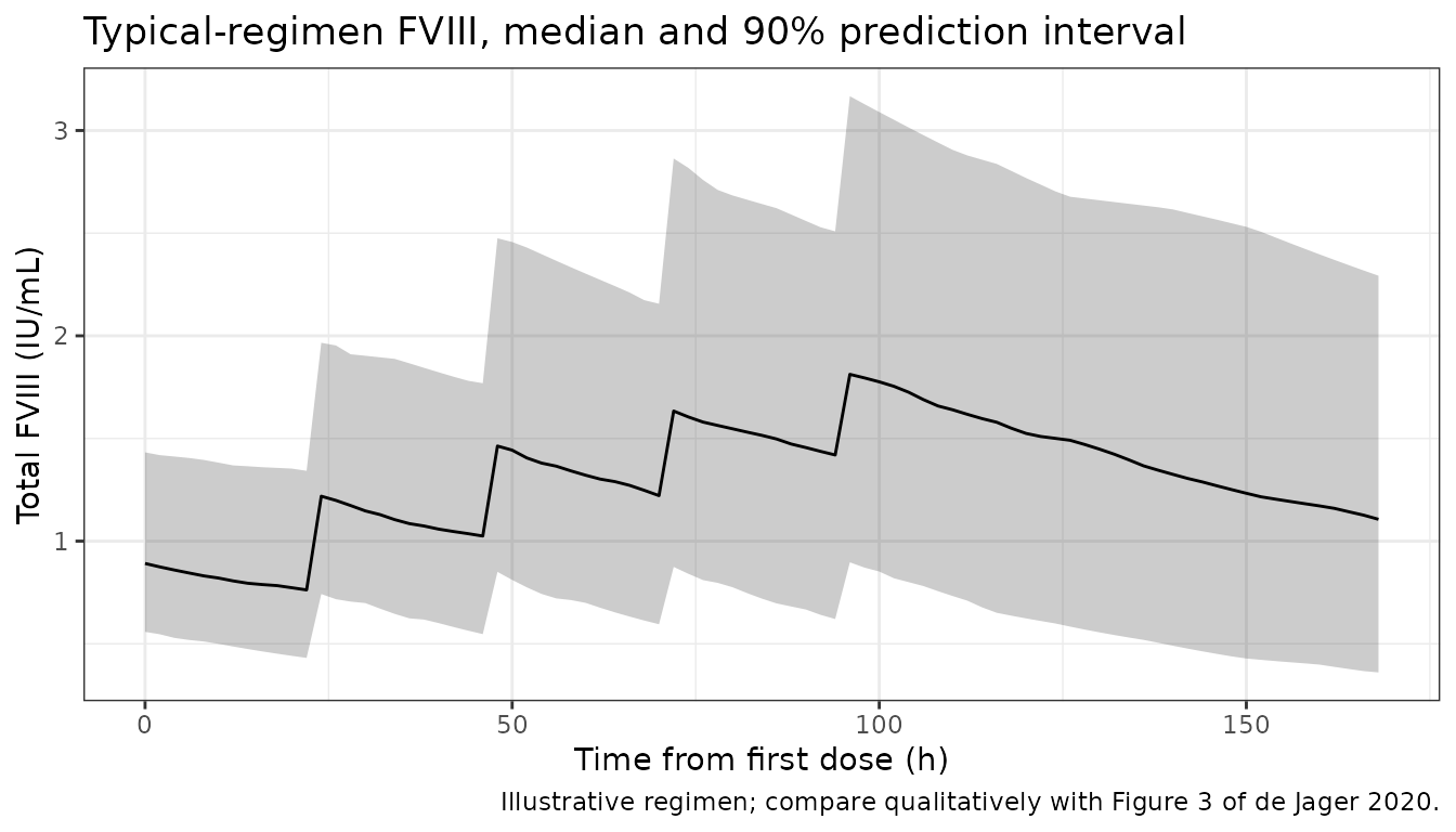
The virtual dose
The packaged model takes the virtual dose as an ordinary dose record
on virtual, and the user chooses the amount. For a patient
whose pre-dose FVIII is above the lowest-ever value, an amount of
excess (IU/mL) * 1000 * V / F at the pre-dose sample time
reproduces the excess at the typical F. With IOV, the realised F varies
by occasion. The check below is a typical-value solve: it confirms that
the virtual contribution enters with F = 0.200 and decays at the same
rate as the concentrate.
vd <- data.frame(id = 1:2, WT = 70, T_SURG = 1.35, VWF = 165, ASA_GE3 = 0, FVIII_BL = 0.41)
amt_virtual <- 0.30 * 1000 * 3.28 / 0.200 # gives +0.30 IU/mL above baseline at time 0
ev_vd <- bind_rows(
  vd |> filter(id == 2) |> mutate(time = 0, evid = 1L, amt = amt_virtual, cmt = "virtual"),
  vd |> tidyr::crossing(time = c(0, 24, 72)) |> mutate(evid = 0L, amt = 0, cmt = "central")
) |>
  arrange(id, time, desc(evid)) |>
  as.data.frame()
sim_vd <- as.data.frame(rxSolve(zeroRe(mod), ev_vd))
#> ℹ parameter labels from comments will be replaced by 'label()'
#> ℹ omega/sigma items treated as zero: 'etalcl', 'etalvc', 'etaiov_lfvirtual_1'
#> Warning: multi-subject simulation without without 'omega'
kel_ref <- typ_cl(70, 81, 1.65, 0) / typ_v(70)
sim_vd |>
  select(id, time, Cc) |>
  tidyr::pivot_wider(names_from = id, values_from = Cc, names_prefix = "id") |>
  mutate(expected_excess = 0.30 * exp(-kel_ref * time), simulated_excess = id2 - id1) |>
  dplyr::rename(
    "Time (h)" = time,
    "No virtual dose (IU/mL)" = id1,
    "With virtual dose (IU/mL)" = id2,
    "Expected excess (IU/mL)" = expected_excess,
    "Simulated excess (IU/mL)" = simulated_excess
  ) |>
knitr::kable(digits = 4, caption = "Typical FVIII with and without a virtual dose at time 0 (baseline 0.41 IU/mL).")| Time (h) | No virtual dose (IU/mL) | With virtual dose (IU/mL) | Expected excess (IU/mL) | Simulated excess (IU/mL) |
|---|---|---|---|---|
| 0 | 0.41 | 0.7100 | 0.3000 | 0.3000 |
| 24 | 0.41 | 0.6388 | 0.2288 | 0.2288 |
| 72 | 0.41 | 0.5432 | 0.1332 | 0.1332 |
Assumptions and deviations
-
Covariate units. Surgery duration is supplied in
hours (
T_SURG), so the 81 min reference becomes 1.35 h. VWF activity is supplied in IU/dL (VWF), so the 1.65 IU/mL reference becomes 165 IU/dL. Both conversions leave the printed effects unchanged. - Text versus equation. Results 3.2 quotes 38% and 29% CL decreases over the interquartile ranges of surgery duration and VWF activity. The final Table 2 exponents give 30% and 24%. No exponent printed anywhere in Table 2 gives the quoted numbers. The model uses the printed equation. The Discussion also gives the RSE of the VWF effect as 51%, while Table 2 shows 43.2% for the final model and 47.1% for the bootstrap.
-
Time-varying VWF activity. The paper carries
measured VWF:Act forward from each measurement to the next. Periods
before the first dose, with a virtual dose, were handled separately; the
paper does not say how. The virtual cohort holds VWF:Act constant per
occasion. A user with measured VWF:Act should supply it as a
time-varying
VWFcolumn. -
Virtual dose. The amount is not reported. The
fitted F and its IOV are kept, and the dose is a user-supplied record on
the paper-specific
virtualstate, eliminated at the same rate ascentral. The simulations above use no virtual dose except in the dedicated check. -
Inter-occasion variability as one eta. The IOV on F
is carried as a single eta,
etaiov_lfvirtual_1. That is exact when each simulated subject represents one surgical occasion. For a patient with several surgeries, simulate each occasion as its own subject. -
Lowest-ever FVIII baseline. The baseline is the
lowest FVIII ever measured in the patient (Methods 2.1), not the most
recent untreated value. The maintainers therefore registered it as
FVIII_BL, separate fromFVIIIRECENT. - ASA class. Only classes II-IV occurred, so the indicator compares ASA III/IV with ASA II. The model has not been informed by ASA I or V patients.
- Virtual cohort. Covariate distributions were chosen to match the Table 1 medians and ranges, with log-normal shapes assumed. The cohort is adult weight only, while the source included seven children.
- Errata. No correction notice for this article was found as of 2026-10-16.