Rifampicin exposure and tuberculous meningitis mortality (Svensson 2020)
Source:vignettes/articles/Svensson_2020_rifampicin.Rmd
Svensson_2020_rifampicin.RmdModel and source
- Citation: Svensson EM, Dian S, te Brake L, Ganiem AR, Yunivita V, van Laarhoven A, van Crevel R, Ruslami R, Aarnoutse RE (2020). Model-Based Meta-analysis of Rifampicin Exposure and Mortality in Indonesian Tuberculous Meningitis Trials. Clin Infect Dis 71(8):1817-1823. doi:10.1093/cid/ciz1071. Parameter estimates from Online Data Supplement Table E1 and the commented NONMEM control stream reproduced in the same supplement (‘NONMEM code pharmacokinetic model’), which also carries the model equations. The saturable-hepatic-extraction structure follows Chirehwa et al. (2016) Antimicrob Agents Chemother 60(1):487-494 doi:10.1128/AAC.01084-15; the transit absorption follows Savic et al. (2007) J Pharmacokinet Pharmacodyn 34(5):711-726.
- Article: https://doi.org/10.1093/cid/ciz1071 (open access, PMC7643733)
- Supplement: the Online Data Supplement to the same DOI carries Table E1 (PK parameter estimates), Tables E2-E3 (survival-model selection) and the commented NONMEM control streams for both the PK and the survival model.
Svensson 2020 pooled individual patient data from three Indonesian phase 2 trials of intensified rifampicin for tuberculous meningitis (TBM) – oral 450 mg (about 10 mg/kg) against 750, 900 or 1350 mg orally or 600 mg as a 1.5 h intravenous infusion – and built two sequential models:
-
Svensson_2020_rifampicin– a population PK model for plasma and lumbar cerebrospinal fluid (CSF). Oral absorption is a Savic transit chain into a liver compartment, elimination is a well-stirred liver with saturable intrinsic clearance, autoinduction is a step change between the first (day 2 +/- 1) and second (day 12 +/- 4) PK occasions, and CSF is an effect compartment whose partition coefficient rises with CSF protein. -
Svensson_2020_rifampicin_survival– a parametric time-to-event model for 6-month mortality with an exponentially declining hazard, effects of baseline Glasgow Coma Scale (GCS) and age, and an Emax reduction by the individual day-2 plasma AUC0-24 predicted by model 1.
The two were fitted separately (the individual AUC is a fixed input
to the survival fit), so they ship as two files that share this article.
The survival model’s AUC covariate AUC_RIF is produced by
simulating the PK model, as shown below.
mod_pk <- readModelDb("Svensson_2020_rifampicin")
mod_tte <- readModelDb("Svensson_2020_rifampicin_survival")
ui_pk <- rxode2::rxode(mod_pk)
#> ℹ parameter labels from comments will be replaced by 'label()'
#> Warning: some etas defaulted to non-mu referenced, possible parsing error: etaiov_cl_1, etaiov_cl_2, etaiov_mtt_1, etaiov_mtt_2, etaiov_logitfdepot_1, etaiov_logitfdepot_2
#> as a work-around try putting the mu-referenced expression on a simple line
ui_tte <- rxode2::rxode(mod_tte)
mod_pk_typ <- rxode2::zeroRe(ui_pk)
#> Warning: some etas defaulted to non-mu referenced, possible parsing error: etaiov_cl_1, etaiov_cl_2, etaiov_mtt_1, etaiov_mtt_2, etaiov_logitfdepot_1, etaiov_logitfdepot_2
#> as a work-around try putting the mu-referenced expression on a simple line

# The Savic analytical transit input must not be auto-solved away.
stopifnot(is.null(ui_pk$linCmt))
Population
The pooled cohort (Table 1) was 148 adults, median age 30 years (16-81), median weight 46 kg (34-78), 45% female, 12% HIV-infected, 56% with definite TBM and 95% with grade 2 or 3 disease; baseline GCS median 13 (3-15) and CSF total protein median 165 mg/dL (9-3869). The PK analysis used the 133 patients with PK data (1150 concentrations, 170 from CSF); the survival analysis used all 148 (58 deaths, 15 dropouts within 6 months). All three trials were run in Bandung, Indonesia.
Source trace
| Model element | Value used | Source location |
|---|---|---|
| CLint,max | 40.468 L/h | Table E1 (40.5); control stream $THETA 1 |
| Km | 16.1378 mg/L | Table E1 (16.1); $THETA 2 |
| V | 7.37836 L | Table E1 (7.38); $THETA 3 |
| ka | 1.40998 1/h | Table E1 (1.41); $THETA 4 |
| MTT | 0.672668 h | Table E1 (0.67); $THETA 5 |
| Number of transit compartments | 4.23047 | Table E1 (4.23); $THETA 6 |
| Prehepatic bioavailability | 0.77584 (logit scale) | Table E1 (77.6%); $THETA 7; $PK
PHI/BIO |
| Induction on CLint,max at occasion 2 | +48.0% | Table E1 (47.9%, footnote a); $THETA 8 |
| Volume change at occasion 2 | -19.257% (V and Vp) | Table E1 (-19.3%); $THETA 9 |
| Q | 93.1391 L/h | Table E1 (93.1); $THETA 10 |
| Vp | 26.2304 L | Table E1 (26.2); $THETA 11 |
| CSF equilibration half-life | 2.06319 h (ke0 = log(2)/2.06319) | Table E1 (2.07); $THETA 12 |
| CSF partition coefficient | 0.0544996 | Table E1 (5.46%); $THETA 13 |
| CSF protein effect | 0.630943 | Table E1 (63.1%, footnote b); $THETA 14 |
| QH, VH, fu | 50 L/h, 1 L, 0.2 (fixed) | Supplement “Pharmacokinetic model”; $PK
|
| IV infusion duration | 1.5 h (fixed) | Main text Methods; $PK D3 |
| FFM allometry | exponents 0.75 / 1, reference 44.55 kg | Supplement; $PK ALLMCL / ALLMV |
| IIV / IOV variances | 0.0598 (CL IOV), 1.145 (V), 0.576 (ka), 0.379 (MTT IOV), 1.033 (logit F IOV), 0.948 (Q), 0.125 (PC) | Table E1 (as %CV); $OMEGA
|
| Residual error | plasma 0.1003 mg/L + 23.9%; CSF 0.187 mg/L | Table E1; $SIGMA
|
| Liver, transit, CSF ODEs |
$DES DADT(1)-DADT(5) |
Supplement control stream |
| Base hazard | 0.0285801 1/day | Table 2 (0.0286); survival $THETA 1 |
| Hazard decline rate | 0.0333392 1/day | Table 2 (0.0333); $THETA 2 |
| GCS effect | -0.255676 per point | Table 2 (-0.256); $THETA 3 |
| Age exponent | 1.0438 | Table 2 (1.04); $THETA 4 |
| AUC50 of the rifampicin effect | 171.358 mg*h/L | Table 2 (171); $THETA 5 |
| Hazard equation | h(t) = BASE e^(-kt) (1 + thGCS (GCS - 13)) (age/30)^thage (1 - AUC/(AUC50 + AUC)) | Table 2 footnote a; survival $DES
|
Encoding checks
Table E1 reports the between-subject and between-occasion
variabilities as sqrt(exp(omega^2) - 1). Recomputing that
from the variances in the model reproduces every printed percentage to
within 0.6 percentage points, which confirms both that the control
stream’s $OMEGA block is the final vector and that the
variances are carried on the right scale.
om <- ui_pk$omega
cv <- function(nm) 100 * sqrt(exp(om[nm, nm]) - 1)
omega_tab <- data.frame(
  eta = c("etaiov_cl_1", "etalvc", "etalka", "etaiov_mtt_1",
          "etaiov_logitfdepot_1", "etalq", "etalppc"),
  printed = c(24.8, 147, 88.3, 67.7, 134, 126, 36.3)
)
omega_tab$recomputed <- vapply(omega_tab$eta, cv, numeric(1))
knitr::kable(omega_tab, digits = 1)| eta | printed | recomputed |
|---|---|---|
| etaiov_cl_1 | 24.8 | 24.8 |
| etalvc | 147.0 | 146.4 |
| etalka | 88.3 | 88.3 |
| etaiov_mtt_1 | 67.7 | 67.9 |
| etaiov_logitfdepot_1 | 134.0 | 134.5 |
| etalq | 126.0 | 125.7 |
| etalppc | 36.3 | 36.4 |
stopifnot(all(abs(omega_tab$recomputed - omega_tab$printed) < 0.6))

# The proportional residual error follows the same convention:
# sqrt(exp(0.0572954) - 1) = 24.3% (Table E1), while the SD is 23.9%.
prop_sd <- ui_pk$theta[["propSd"]]
stopifnot(abs(100 * sqrt(exp(prop_sd^2) - 1) - 24.3) < 0.05)

# ke0 is the library's canonical rate constant; the paper uses a half-life.
stopifnot(abs(log(2) / exp(ui_pk$theta[["lke0"]]) - 2.06319) < 1e-6)
Structural validation of the PK model
Simulation helper
The PK model has two error endpoints (Cc and
Ccsf), so observation rows carry dvid = 1;
rxode2 then returns both observables as columns.
make_events <- function(ids, dose, route, ffm, occ = 1, csf_tpro = 1.65,
                        dose_times = c(0, 24), obs_times = seq(0, 48, by = 0.25)) {
  dose_rows <- expand.grid(id = ids, time = dose_times) |>
    dplyr::mutate(amt = dose, evid = 1L, dvid = NA_integer_,
                  cmt = if (route == "iv") "central" else "depot",
                  rate = if (route == "iv") -2 else 0)
  obs_rows <- expand.grid(id = ids, time = obs_times) |>
    dplyr::mutate(amt = NA_real_, evid = 0L, dvid = 1L, cmt = NA_character_, rate = 0)
  ev <- dplyr::bind_rows(dose_rows, obs_rows) |>
    dplyr::arrange(id, time, dplyr::desc(evid))
  ev$FFM <- if (length(ffm) == 1) ffm else ffm[match(ev$id, ids)]
  ev$OCC <- occ
  ev$CSF_TPRO <- csf_tpro
  ev
}

trapz <- function(x, y) sum(diff(x) * (head(y, -1) + tail(y, -1)) / 2)
Mass balance
With the random effects set to zero, all drug that enters the liver
is eventually eliminated there, so the integral of the hepatic
elimination flux clh / vh * liver must equal the
bioavailable dose: F * Dose after an oral dose and
Dose after the infusion. This also proves the Savic transit
input is live (a silently zeroed input would give 0).
mb_times <- sort(unique(c(seq(0, 3, by = 0.005), seq(3, 150, by = 0.05))))
f_typ <- plogis(ui_pk$theta[["logitfdepot"]])
mb <- lapply(list(c(450, 0), c(1350, 0), c(600, 1)), function(x) {
  ev <- make_events(1, x[1], if (x[2] == 1) "iv" else "oral", ffm = 44.55,
                    dose_times = 0, obs_times = mb_times)
  s <- as.data.frame(rxode2::rxSolve(mod_pk_typ, ev))
  data.frame(dose = x[1], route = if (x[2] == 1) "IV" else "oral",
             eliminated = trapz(s$time, s$clh / s$vh * s$liver),
             expected = x[1] * if (x[2] == 1) 1 else f_typ,
             max_depot = max(s$depot))
})
#> ℹ omega/sigma items treated as zero: 'etaiov_cl_1', 'etaiov_cl_2', 'etalvc', 'etalka', 'etaiov_mtt_1', 'etaiov_mtt_2', 'etaiov_logitfdepot_1', 'etaiov_logitfdepot_2', 'etalq', 'etalppc'
#> ℹ omega/sigma items treated as zero: 'etaiov_cl_1', 'etaiov_cl_2', 'etalvc', 'etalka', 'etaiov_mtt_1', 'etaiov_mtt_2', 'etaiov_logitfdepot_1', 'etaiov_logitfdepot_2', 'etalq', 'etalppc'
#> ℹ omega/sigma items treated as zero: 'etaiov_cl_1', 'etaiov_cl_2', 'etalvc', 'etalka', 'etaiov_mtt_1', 'etaiov_mtt_2', 'etaiov_logitfdepot_1', 'etaiov_logitfdepot_2', 'etalq', 'etalppc'
mb <- dplyr::bind_rows(mb) |> dplyr::mutate(ratio = eliminated / expected)
knitr::kable(mb, digits = 4)| dose | route | eliminated | expected | max_depot | ratio |
|---|---|---|---|---|---|
| 450 | oral | 349.1286 | 349.128 | 178.944 | 1 |
| 1350 | oral | 1047.3831 | 1047.384 | 536.832 | 1 |
| 600 | IV | 600.0007 | 600.000 | 0.000 | 1 |
Saturable clearance and autoinduction
Typical-value day-2 AUC0-24 (the second daily dose, 24-48 h) at the reference fat-free mass of 44.55 kg. Saturable hepatic extraction makes exposure rise more than proportionally with dose, and the step induction at occasion 2 (CLint,max +48%, volumes -19%) lowers exposure at the same dose.
typ_auc <- function(dose, route, occ = 1, ffm = 44.55) {
  s <- as.data.frame(rxode2::rxSolve(
    mod_pk_typ, make_events(1, dose, route, ffm = ffm, occ = occ,
                            obs_times = seq(0, 48, by = 0.02))
  ))
  s <- s[s$time >= 24, ]
  trapz(s$time, s$Cc)
}
typ_tab <- data.frame(
  regimen = c("450 mg oral", "600 mg IV", "750 mg oral", "900 mg oral", "1350 mg oral"),
  dose = c(450, 600, 750, 900, 1350),
  route = c("oral", "iv", "oral", "oral", "oral"),
  # Typical exposures the survival control stream imputes for the 15 patients
  # without PK data ("IF(RIFAUC.EQ.-99.AND.RIFDOSE.EQ.450) RIFAUC = 47.61" ...).
  imputed_in_source = c(47.61, 119.1, 123.1, 183, 233)
)
typ_tab$auc_occ1 <- mapply(typ_auc, typ_tab$dose, typ_tab$route)
#> ℹ omega/sigma items treated as zero: 'etaiov_cl_1', 'etaiov_cl_2', 'etalvc', 'etalka', 'etaiov_mtt_1', 'etaiov_mtt_2', 'etaiov_logitfdepot_1', 'etaiov_logitfdepot_2', 'etalq', 'etalppc'
#> ℹ omega/sigma items treated as zero: 'etaiov_cl_1', 'etaiov_cl_2', 'etalvc', 'etalka', 'etaiov_mtt_1', 'etaiov_mtt_2', 'etaiov_logitfdepot_1', 'etaiov_logitfdepot_2', 'etalq', 'etalppc'
#> ℹ omega/sigma items treated as zero: 'etaiov_cl_1', 'etaiov_cl_2', 'etalvc', 'etalka', 'etaiov_mtt_1', 'etaiov_mtt_2', 'etaiov_logitfdepot_1', 'etaiov_logitfdepot_2', 'etalq', 'etalppc'
#> ℹ omega/sigma items treated as zero: 'etaiov_cl_1', 'etaiov_cl_2', 'etalvc', 'etalka', 'etaiov_mtt_1', 'etaiov_mtt_2', 'etaiov_logitfdepot_1', 'etaiov_logitfdepot_2', 'etalq', 'etalppc'
#> ℹ omega/sigma items treated as zero: 'etaiov_cl_1', 'etaiov_cl_2', 'etalvc', 'etalka', 'etaiov_mtt_1', 'etaiov_mtt_2', 'etaiov_logitfdepot_1', 'etaiov_logitfdepot_2', 'etalq', 'etalppc'
typ_tab$auc_occ2 <- mapply(typ_auc, typ_tab$dose, typ_tab$route, MoreArgs = list(occ = 2))
#> ℹ omega/sigma items treated as zero: 'etaiov_cl_1', 'etaiov_cl_2', 'etalvc', 'etalka', 'etaiov_mtt_1', 'etaiov_mtt_2', 'etaiov_logitfdepot_1', 'etaiov_logitfdepot_2', 'etalq', 'etalppc'
#> ℹ omega/sigma items treated as zero: 'etaiov_cl_1', 'etaiov_cl_2', 'etalvc', 'etalka', 'etaiov_mtt_1', 'etaiov_mtt_2', 'etaiov_logitfdepot_1', 'etaiov_logitfdepot_2', 'etalq', 'etalppc'
#> ℹ omega/sigma items treated as zero: 'etaiov_cl_1', 'etaiov_cl_2', 'etalvc', 'etalka', 'etaiov_mtt_1', 'etaiov_mtt_2', 'etaiov_logitfdepot_1', 'etaiov_logitfdepot_2', 'etalq', 'etalppc'
#> ℹ omega/sigma items treated as zero: 'etaiov_cl_1', 'etaiov_cl_2', 'etalvc', 'etalka', 'etaiov_mtt_1', 'etaiov_mtt_2', 'etaiov_logitfdepot_1', 'etaiov_logitfdepot_2', 'etalq', 'etalppc'
#> ℹ omega/sigma items treated as zero: 'etaiov_cl_1', 'etaiov_cl_2', 'etalvc', 'etalka', 'etaiov_mtt_1', 'etaiov_mtt_2', 'etaiov_logitfdepot_1', 'etaiov_logitfdepot_2', 'etalq', 'etalppc'
knitr::kable(typ_tab |> dplyr::select(-route) |>
               dplyr::rename("Regimen" = regimen, "Dose (mg)" = dose,
                             "Imputed AUC in source (mg*h/L)" = imputed_in_source,
                             "Typical AUC, occasion 1" = auc_occ1,
                             "Typical AUC, occasion 2" = auc_occ2),
digits = 1)| Regimen | Dose (mg) | Imputed AUC in source (mg*h/L) | Typical AUC, occasion 1 | Typical AUC, occasion 2 |
|---|---|---|---|---|
| 450 mg oral | 450 | 47.6 | 56.5 | 39.2 |
| 600 mg IV | 600 | 119.1 | 124.5 | 91.2 |
| 750 mg oral | 750 | 123.1 | 109.5 | 76.8 |
| 900 mg oral | 900 | 183.0 | 140.9 | 99.2 |
| 1350 mg oral | 1350 | 233.0 | 256.1 | 181.1 |
oral <- typ_tab[typ_tab$route == "oral", ]
# More than dose-proportional: 3-fold dose gives > 3-fold AUC.
stopifnot(oral$auc_occ1[oral$dose == 1350] / oral$auc_occ1[oral$dose == 450] > 3.5)
# Induction lowers exposure at every dose.
stopifnot(all(typ_tab$auc_occ2 < typ_tab$auc_occ1))
# The intravenous regimen carries no bioavailability variability, so its
# imputed value is the cleanest comparison with a typical-value solve.
iv_ratio <- typ_tab$auc_occ1[typ_tab$route == "iv"] / typ_tab$imputed_in_source[typ_tab$route == "iv"]
stopifnot(abs(iv_ratio - 1) < 0.15)
The imputed values in the survival control stream are “typical exposures imputed based on the model, patient characteristics, and the given dose”, so they depend on the characteristics of the patients in each dose group, which are not published. The intravenous value (124.5 simulated against 119.1 mg*h/L imputed) agrees within 5%. The oral imputed values scatter around the typical-value solve in both directions (below it at 450 mg, above it at 900 mg), which a single systematic error could not produce.
CSF partition
At steady state the CSF concentration tracks PC * Cc
with a 2.06 h lag. Integrated over a long profile,
AUC_CSF / AUC_plasma must equal the partition coefficient
exactly, and a CSF protein of 16.5 g/L (ten times the median) raises it
by 0.631 / log10(165) = 28.5% under the as-run
equation.
csf_ratio <- function(prot) {
  s <- as.data.frame(rxode2::rxSolve(
    mod_pk_typ, make_events(1, 900, "oral", ffm = 44.55, csf_tpro = prot,
                            dose_times = 0, obs_times = seq(0, 150, by = 0.02))
  ))
  trapz(s$time, s$Ccsf) / trapz(s$time, s$Cc)
}
r_med <- csf_ratio(1.65)
#> ℹ omega/sigma items treated as zero: 'etaiov_cl_1', 'etaiov_cl_2', 'etalvc', 'etalka', 'etaiov_mtt_1', 'etaiov_mtt_2', 'etaiov_logitfdepot_1', 'etaiov_logitfdepot_2', 'etalq', 'etalppc'
r_hi <- csf_ratio(16.5)
#> ℹ omega/sigma items treated as zero: 'etaiov_cl_1', 'etaiov_cl_2', 'etalvc', 'etalka', 'etaiov_mtt_1', 'etaiov_mtt_2', 'etaiov_logitfdepot_1', 'etaiov_logitfdepot_2', 'etalq', 'etalppc'
c(median_protein = r_med, tenfold_protein = r_hi, ratio = r_hi / r_med)
#>  median_protein tenfold_protein           ratio
#>      0.05449960      0.07000643      1.28453103
stopifnot(abs(r_med / exp(ui_pk$theta[["lppc"]]) - 1) < 1e-3)
stopifnot(abs(r_hi / r_med - (1 + 0.630943 / log10(165))) < 1e-3)
Virtual cohort
Table 3 of the paper evaluates target attainment for 450-1800 mg in 10,000 virtual patients whose sex, weight and height were resampled from a large Indonesian TBM cohort plus an African pulmonary TB cohort. Those data are not published, so this cohort draws weight from a log-normal distribution with the Table 1 median (46 kg), restricted to the Table 1 range by redrawing, 45% female, and assumed Indonesian adult heights; fat-free mass follows Janmahasatian 2005. The paper does not state which FFM formula it used.
set.seed(2020)
n_per_arm <- 200
draw_cohort <- function(n) {
  wt <- numeric(0)
  while (length(wt) < n) {
    w <- exp(rnorm(n, log(46), 0.18))
    wt <- c(wt, w[w >= 34 & w <= 78])
  }
  wt <- wt[seq_len(n)]
  sexf <- rbinom(n, 1, 0.45)
  ht <- ifelse(sexf == 1, rnorm(n, 1.52, 0.06), rnorm(n, 1.63, 0.06))
  bmi <- wt / ht^2
  ffm <- ifelse(sexf == 1, 9270 * wt / (8780 + 244 * bmi), 9270 * wt / (6680 + 216 * bmi))
  data.frame(wt = wt, sexf = sexf, ht = ht, ffm = ffm)
}
cohort <- draw_cohort(n_per_arm)
summary(cohort$ffm)
#>    Min. 1st Qu.  Median    Mean 3rd Qu.    Max.
#>   25.80   32.91   38.66   38.49   43.19   55.82
stopifnot(abs(median(cohort$wt) - 46) < 3)
Simulation
Each arm receives two once-daily oral doses on the first PK occasion
(OCC = 1); the day-2 AUC0-24 is the 24-48 h interval. The
same virtual patients are used in every arm, as in the paper (“using the
same seed number for all evaluated doses”).
doses <- c(450, 900, 1350, 1800)
rxode2::rxSetSeed(2020)
sim <- lapply(seq_along(doses), function(k) {
  ids <- (k - 1) * n_per_arm + seq_len(n_per_arm)
  ev <- make_events(ids, doses[k], "oral", ffm = cohort$ffm)
  s <- as.data.frame(rxode2::rxSolve(ui_pk, ev, keep = "FFM"))
  s$treatment <- paste(doses[k], "mg")
  s$dose <- doses[k]
  s
}) |> dplyr::bind_rows()
sim$treatment <- factor(sim$treatment, levels = paste(doses, "mg"))
sim |>
  dplyr::group_by(treatment, time) |>
  dplyr::summarise(med = median(ipredSim), lo = quantile(ipredSim, 0.05),
                   hi = quantile(ipredSim, 0.95), .groups = "drop") |>
  ggplot(aes(time, med, colour = treatment, fill = treatment)) +
  geom_ribbon(aes(ymin = lo, ymax = hi), alpha = 0.15, colour = NA) +
  geom_line() +
  labs(x = "Time after first dose (h)", y = "Rifampicin plasma concentration (mg/L)",
       colour = "Dose", fill = "Dose") +
  theme_bw()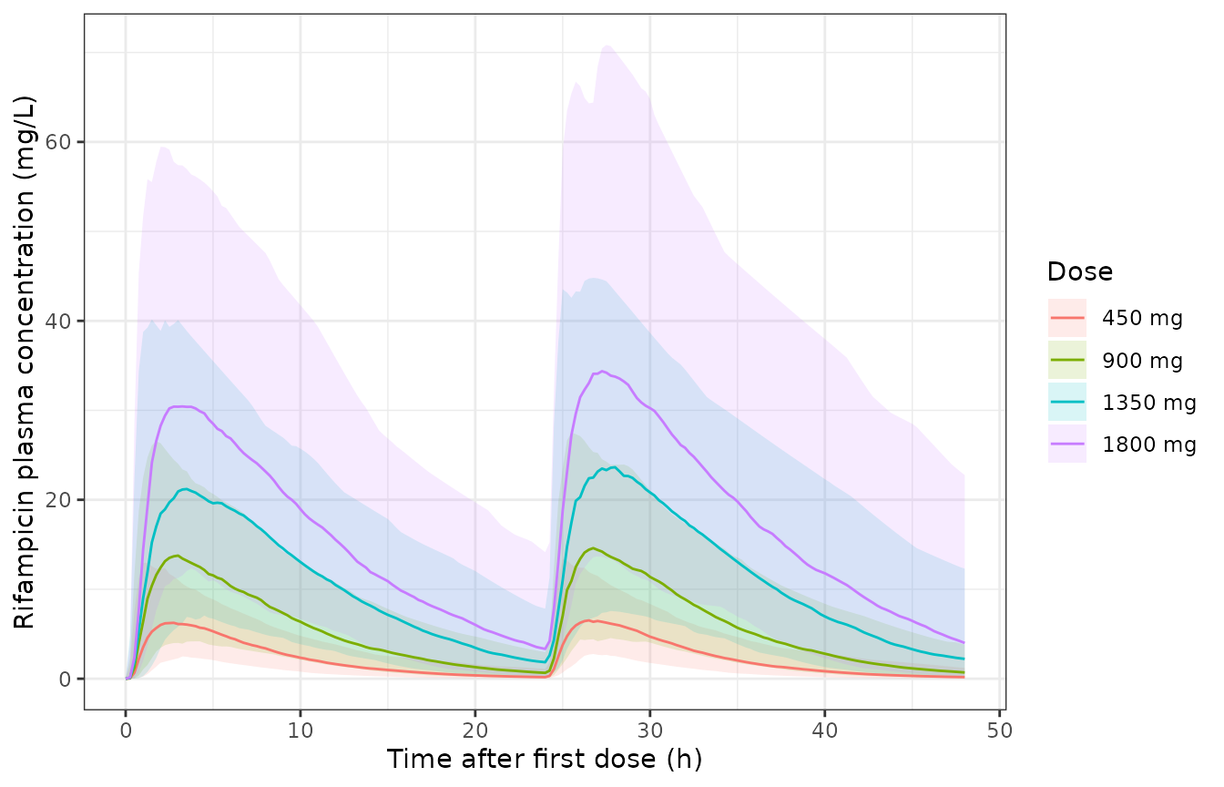
Simulated day-1 and day-2 plasma rifampicin (individual predictions without residual error): median and 5th-95th percentiles per dose.
PKNCA validation
sim_nca <- sim |>
  dplyr::select(id, treatment, time, conc = ipredSim) |>
  dplyr::filter(!is.na(conc))
dose_df <- sim |>
  dplyr::distinct(id, treatment, dose) |>
  tidyr::crossing(time = c(0, 24)) |>
  dplyr::rename(amt = dose)
conc_obj <- PKNCA::PKNCAconc(sim_nca, conc ~ time | treatment + id,
                             concu = "mg/L", timeu = "h")
dose_obj <- PKNCA::PKNCAdose(dose_df, amt ~ time | treatment + id,
                             doseu = "mg", route = "extravascular")
intervals <- data.frame(start = 24, end = 48, cmax = TRUE, tmax = TRUE, auclast = TRUE)
nca <- PKNCA::pk.nca(PKNCA::PKNCAdata(conc_obj, dose_obj, intervals = intervals))
nca_res <- as.data.frame(nca$result)

auc2 <- nca_res |>
  dplyr::filter(PPTESTCD == "auclast") |>
  dplyr::select(treatment, id, auc = PPORRES)
stopifnot(nrow(auc2) == length(doses) * n_per_arm, !anyNA(auc2$auc))

# Test the instrument: PKNCA's AUC must agree with a direct trapezoid.
direct <- sim |>
  dplyr::filter(time >= 24, time <= 48) |>
  dplyr::group_by(treatment, id) |>
  dplyr::summarise(auc_direct = trapz(time, ipredSim), .groups = "drop") |>
  dplyr::inner_join(auc2, by = c("treatment", "id"))
stopifnot(abs(median(direct$auc / direct$auc_direct) - 1) < 0.01)

summary(nca)
#>  Interval Start Interval End treatment   N AUClast (h*mg/L) Cmax (mg/L)
#>              24           48    450 mg 200      57.0 [51.0] 7.13 [50.9]
#>              24           48    900 mg 200       135 [59.5] 14.4 [60.4]
#>              24           48   1350 mg 200       266 [61.9] 23.7 [54.0]
#>              24           48   1800 mg 200       426 [63.6] 35.6 [53.8]
#>            Tmax (h)
#>  2.50 [0.500, 7.50]
#>  2.50 [0.750, 6.75]
#>  3.00 [0.500, 10.0]
#>  3.00 [0.500, 8.75]
#>
#> Caption: AUClast, Cmax: geometric mean and geometric coefficient of variation; Tmax: median and range; N: number of subjects
Comparison with Table 3 (probability of target attainment)
pta <- auc2 |>
  dplyr::group_by(treatment) |>
  dplyr::summarise(median_auc = median(auc),
                   sim_171 = 100 * mean(auc > 171),
                   sim_300 = 100 * mean(auc > 300), .groups = "drop") |>
  dplyr::mutate(paper_171 = c(0.47, 67.8, 97.6, 99.8),
                paper_300 = c(0, 11.4, 70.1, 94.5))
pta |>
  dplyr::rename("Dose" = treatment, "Median day-2 AUC0-24 (mg*h/L)" = median_auc,
                "P(AUC > 171), simulated %" = sim_171, "P(AUC > 171), Table 3 %" = paper_171,
                "P(AUC > 300), simulated %" = sim_300, "P(AUC > 300), Table 3 %" = paper_300) |>
knitr::kable(digits = 1)| Dose | Median day-2 AUC0-24 (mg*h/L) | P(AUC > 171), simulated % | P(AUC > 300), simulated % | P(AUC > 171), Table 3 % | P(AUC > 300), Table 3 % |
|---|---|---|---|---|---|
| 450 mg | 59.8 | 0.0 | 0.0 | 0.5 | 0.0 |
| 900 mg | 149.6 | 36.0 | 5.5 | 67.8 | 11.4 |
| 1350 mg | 284.6 | 76.5 | 47.5 | 97.6 | 70.1 |
| 1800 mg | 437.8 | 93.5 | 75.0 | 99.8 | 94.5 |
# Centre-of-distribution gates, robust to which subjects land in the tails.
stopifnot(
  all(diff(pta$median_auc) > 0),
  pta$sim_171[1] < 5,
  pta$sim_171[4] > 80
)
The simulated attainment runs below Table 3 at 900 and 1350 mg. Two causes were identified while building this article, neither resolvable from the published material:
- The virtual population. Exposure depends strongly on fat-free mass through the saturable liver, and the paper’s resampled Indonesian + African population is not published. Lowering the FFM of the cohort raises the 900 and 1350 mg attainment toward the Table 3 values.
- Between-occasion variability. The model carries large between-occasion variability in bioavailability (134% on the logit scale), which widens the AUC distribution. Rerunning the same cohort with the between-occasion variances set to zero (below) gives the narrow spread of Table 3 at the highest dose. This suggests that the paper’s simulation drew between-subject but not between-occasion variability, which the paper does not state.
ui_pk_noiov <- ui_pk |>
  rxode2::ini(etaiov_cl_1 = 0, etaiov_mtt_1 = 0, etaiov_logitfdepot_1 = 0)
#> ℹ change initial estimate of `etaiov_cl_1` to `0`
#> ℹ change initial estimate of `etaiov_mtt_1` to `0`
#> ℹ change initial estimate of `etaiov_logitfdepot_1` to `0`
rxode2::rxSetSeed(2020)
auc_noiov <- lapply(seq_along(doses), function(k) {
  ids <- (k - 1) * n_per_arm + seq_len(n_per_arm)
  ev <- make_events(ids, doses[k], "oral", ffm = cohort$ffm)
  s <- as.data.frame(rxode2::rxSolve(ui_pk_noiov, ev))
  s <- s[s$time >= 24, ]
  data.frame(treatment = paste(doses[k], "mg"),
             auc = vapply(split(s, s$id), function(d) trapz(d$time, d$ipredSim), numeric(1)))
}) |> dplyr::bind_rows()
#> ℹ omega/sigma items treated as zero: 'etaiov_cl_1', 'etaiov_mtt_1', 'etaiov_logitfdepot_1'
#> ℹ omega/sigma items treated as zero: 'etaiov_cl_1', 'etaiov_mtt_1', 'etaiov_logitfdepot_1'
#> ℹ omega/sigma items treated as zero: 'etaiov_cl_1', 'etaiov_mtt_1', 'etaiov_logitfdepot_1'
#> ℹ omega/sigma items treated as zero: 'etaiov_cl_1', 'etaiov_mtt_1', 'etaiov_logitfdepot_1'
pta_noiov <- auc_noiov |>
  dplyr::mutate(treatment = factor(treatment, levels = paste(doses, "mg"))) |>
  dplyr::group_by(treatment) |>
  dplyr::summarise(median_auc = median(auc), sim_171 = 100 * mean(auc > 171),
                   sim_300 = 100 * mean(auc > 300), .groups = "drop") |>
  dplyr::mutate(paper_171 = c(0.47, 67.8, 97.6, 99.8),
                paper_300 = c(0, 11.4, 70.1, 94.5))
pta_noiov |>
  dplyr::rename("Dose" = treatment, "Median day-2 AUC0-24 (mg*h/L)" = median_auc,
                "P(AUC > 171), no IOV %" = sim_171, "P(AUC > 171), Table 3 %" = paper_171,
                "P(AUC > 300), no IOV %" = sim_300, "P(AUC > 300), Table 3 %" = paper_300) |>
knitr::kable(digits = 1)| Dose | Median day-2 AUC0-24 (mg*h/L) | P(AUC > 171), no IOV % | P(AUC > 300), no IOV % | P(AUC > 171), Table 3 % | P(AUC > 300), Table 3 % |
|---|---|---|---|---|---|
| 450 mg | 64.8 | 0.0 | 0.0 | 0.5 | 0.0 |
| 900 mg | 162.9 | 42.0 | 0.0 | 67.8 | 11.4 |
| 1350 mg | 305.5 | 99.5 | 53.0 | 97.6 | 70.1 |
| 1800 mg | 484.1 | 100.0 | 95.5 | 99.8 | 94.5 |
# Without between-occasion variability the 1800 mg arm is almost entirely
# above both targets, as in Table 3, and clearly narrower than with it.
stopifnot(
  pta_noiov$sim_171[4] > 97,
  pta_noiov$sim_300[4] > pta$sim_300[4] + 5
)
Survival model
Replicating Figure 1 (covariate effects on the hazard)
th <- ui_tte$theta
fig1 <- dplyr::bind_rows(
  data.frame(panel = "Age (years)", x = seq(16, 81, length.out = 100)) |>
    dplyr::mutate(rel = (x / 30)^th[["e_age_haz"]]),
  data.frame(panel = "Baseline GCS", x = seq(3, 15, length.out = 100)) |>
    dplyr::mutate(rel = 1 + th[["e_gcs_haz"]] * (x - 13)),
  data.frame(panel = "Day-2 AUC0-24 (mg*h/L)", x = seq(0, 500, length.out = 100)) |>
    dplyr::mutate(rel = 1 - x / (exp(th[["lec50_auc"]]) + x))
)
ggplot(fig1, aes(x, rel)) +
  geom_line() +
  facet_wrap(~panel, scales = "free") +
  labs(x = NULL, y = "Relative hazard") +
  theme_bw()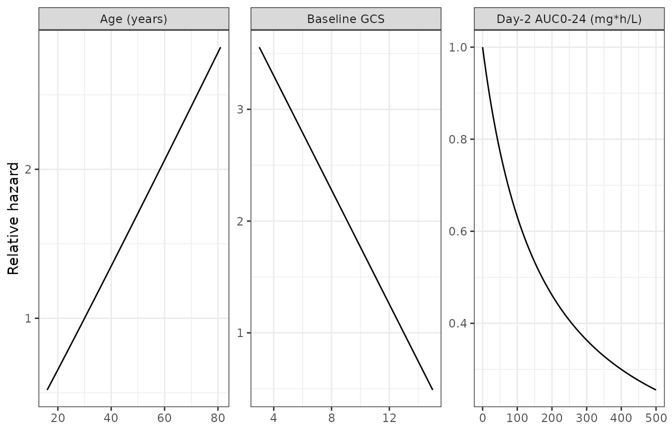
Replicates Figure 1 of Svensson 2020: relative hazard as a function of age (reference 30 years), baseline GCS (reference 13) and day-2 plasma AUC0-24 (relative to no rifampicin), over the observed ranges.
Replicating Figure 2 (typical survival by exposure)
Figure 2 shows model-predicted survival for a typical patient (age
30, baseline GCS 13) at the exposure of each dose group. The exposures
used here are the per-dose typical values imputed in the survival
control stream. The hazard has a closed-form integral,
H(t) = BASE / k * (1 - exp(-k t)) * EFF, which the ODE
solve must match.
fig2_auc <- data.frame(
  group = c("450 mg PO", "600 mg IV", "750 mg PO", "900 mg PO", "1350 mg PO"),
  AUC_RIF = c(47.61, 119.1, 123.1, 183, 233)
)
ev_tte <- expand.grid(id = seq_len(nrow(fig2_auc)), time = seq(0, 180, by = 1)) |>
  dplyr::arrange(id, time) |>
  dplyr::mutate(evid = 0L, cmt = "cumhaz", AGE = 30, SCORE_GCS = 13,
                AUC_RIF = fig2_auc$AUC_RIF[id])
surv <- as.data.frame(rxode2::rxSolve(ui_tte, ev_tte, keep = "AUC_RIF")) |>
  dplyr::mutate(group = factor(fig2_auc$group[id], levels = fig2_auc$group))
#> Warning: multi-subject simulation without without 'omega'

# Closed-form check (same parameters on both sides: pure numerical error).
base <- exp(th[["lbase"]]); kd <- exp(th[["lkdec"]]); ec50 <- exp(th[["lec50_auc"]])
surv$closed <- exp(-base / kd * (1 - exp(-kd * surv$time)) * (1 - surv$AUC_RIF / (ec50 + surv$AUC_RIF)))
stopifnot(max(abs(surv$sur - surv$closed)) < 1e-6)

ggplot(surv, aes(time, sur, colour = group)) +
  geom_line() +
  coord_cartesian(ylim = c(0.4, 1)) +
  labs(x = "Time (days)", y = "Proportion surviving", colour = "Exposure group") +
  theme_bw()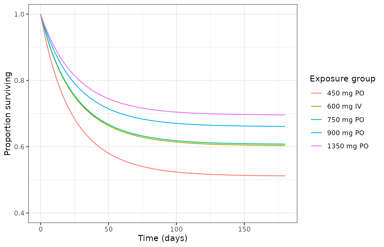
Replicates Figure 2 of Svensson 2020: typical-patient survival over 6 months per day-2 plasma rifampicin exposure.
s180 <- surv |> dplyr::filter(time == 180) |> dplyr::select(group, AUC_RIF, sur)
knitr::kable(s180 |> dplyr::rename("Exposure group" = group,
                                   "Day-2 AUC0-24 (mg*h/L)" = AUC_RIF,
"6-month survival" = sur), digits = 3)| Exposure group | Day-2 AUC0-24 (mg*h/L) | 6-month survival |
|---|---|---|
| 450 mg PO | 47.61 | 0.512 |
| 600 mg IV | 119.10 | 0.604 |
| 750 mg PO | 123.10 | 0.608 |
| 900 mg PO | 183.00 | 0.661 |
| 1350 mg PO | 233.00 | 0.696 |
Linking the two models
To predict survival for a new regimen, simulate the PK model on
occasion 1, take each patient’s 24-48 h AUC as AUC_RIF, and
pass it to the survival model. Using the virtual cohort above (all
patients aged 30 with GCS 13):
linked <- auc2 |>
  dplyr::mutate(AUC_RIF = auc, AGE = 30, SCORE_GCS = 13) |>
  dplyr::group_by(treatment) |>
  dplyr::summarise(
    median_auc = median(AUC_RIF),
    mean_surv_6mo = mean(exp(-base / kd * (1 - exp(-kd * 180)) *
                               (1 - AUC_RIF / (ec50 + AUC_RIF)))),
    .groups = "drop"
  )
knitr::kable(linked |> dplyr::rename("Dose" = treatment,
                                     "Median day-2 AUC0-24 (mg*h/L)" = median_auc,
                                     "Mean predicted 6-month survival" = mean_surv_6mo),
digits = 3)| Dose | Median day-2 AUC0-24 (mg*h/L) | Mean predicted 6-month survival |
|---|---|---|
| 450 mg | 59.761 | 0.532 |
| 900 mg | 149.589 | 0.626 |
| 1350 mg | 284.564 | 0.716 |
| 1800 mg | 437.767 | 0.778 |
Assumptions and deviations
-
Parameter source. Values are the final
$THETA,$OMEGAand$SIGMAvectors of the supplement’s control streams, which match the rounded values of Table E1 and Table 2. Two Table E1 entries differ from the control stream in the last printed digit: induction 47.9% (stream 0.480062) and CSF half-life 2.07 h (stream 2.06319). The stream values are used. -
THETA numbering in the PK control stream. The
printed
$THETAblock has 14 entries, but$PKreads the partition coefficient asTHETA(14)and the protein effect asTHETA(15). The values are mapped by their$THETAcomments and Table E1 labels. -
CSF protein effect. The main text says the
partition coefficient rises by 63% “with each 10-fold change in protein
levels”, and Table E1 footnote b calls 63.1% the “effect of one log10
increase”. The control stream that produced the estimate divides the
log10 deviation by
log10(165), so a 10-fold increase actually raises the coefficient by 0.631 / 2.217 = 28.5%. The model uses the control-stream equation, because that is the equation the estimate belongs to. Table E1 footnote b also gives the median as “165 cells/mL”; it is 165 mg/dL (Table 1). The canonicalCSF_TPROcolumn is in g/L and is converted to mg/dL inside the model. -
Autoinduction and occasions. The control stream
switches induction and the volume change on with its
PERIODcolumn (1 = day 2 +/- 1, 2 = day 12 +/- 4). This is carried asOCC, which also multiplexes the between-occasion etas. For simulation, useOCC = 2from day 4 of treatment onward, as the paper describes. -
Between-occasion variability on clearance
multiplies only the eliminated hepatic flux
(
CLH = EH * QH * exp(eta)), not the(1 - EH)outflow to plasma, exactly as in the control stream. Mass is therefore not conserved through the liver when that eta is non-zero; this is the published model. -
Predose initial conditions. The control stream
initialises the central and peripheral compartments from each patient’s
observed predose concentration (
INITCONC), because patients could have had up to 3 days of rifampicin before enrolment. This is a data-fitting device and is not carried; simulations start drug-free. - Missing-covariate imputation in the control stream (FFM 44.55 kg, CSF protein 165 mg/dL) is not carried; supply both columns.
-
Survival model. The source likelihood is the event
density; there is no residual error, and the
$OMEGA 0 FIXis a placeholder. A placeholder additive error of 0.001 onsurlets nlmixr2 accept the model. The survival model uses days as its time unit; the PK model uses hours. - Safety model not included. The paper’s exposure-safety analysis is a per-study constant probability of at least one adverse event (65% in studies 1-2, 83% in study 3) or serious adverse event (23%), with no significant rifampicin exposure effect (P = .47 and P = 1). With no drug dependence there is no exposure-response model to carry.
- Virtual population for Table 3 is an approximation (see above); heights are assumed (women 1.52 m, men 1.63 m, SD 0.06 m) and FFM uses Janmahasatian 2005.
- Errata. A search on 2026-09-27 found no erratum or correction for this article (Crossref update metadata and Europe PMC).