Darunavir in SARS-CoV-2 and HIV patients (Cojutti 2020)
Source:vignettes/articles/Cojutti_2020_darunavir.Rmd
Cojutti_2020_darunavir.Rmd
mod_covid <- readModelDb("Cojutti_2020_darunavir_covid19")
mod_hiv <- readModelDb("Cojutti_2020_darunavir_hiv")
ui_covid <- rxode2::rxode(mod_covid)
#> ℹ parameter labels from comments will be replaced by 'label()'
ui_hiv <- rxode2::rxode(mod_hiv)
#> ℹ parameter labels from comments will be replaced by 'label()'
Model and source
- Citation: Cojutti PG, Londero A, Della Siega P, Givone F, Fabris M, Biasizzo J, Tascini C, Pea F. Comparative Population Pharmacokinetics of Darunavir in SARS-CoV-2 Patients vs. HIV Patients: The Role of Interleukin-6. Clin Pharmacokinet. 2020;59(10):1251-1260. doi:10.1007/s40262-020-00933-8. PMCID: PMC7453069.
- Article: https://doi.org/10.1007/s40262-020-00933-8
- Open-access full text: https://www.ncbi.nlm.nih.gov/pmc/articles/PMC7453069/
Cojutti and colleagues noticed during the first Italian COVID-19 wave that darunavir trough concentrations in hospitalised SARS-CoV-2 patients were much higher than those usually seen in HIV patients on the same dose. They fitted two separate one-compartment population PK models in Monolix 2019R1 (SAEM), one per population, from routine therapeutic drug monitoring (a trough and a 2 h sample per patient):
-
Cojutti_2020_darunavir_covid19– 30 SARS-CoV-2 patients on darunavir/cobicistat 800/150 mg or darunavir/ritonavir 800/100 mg once daily. Serum interleukin-6 (IL-6) lowers apparent clearance CL/F by a power function, and body surface area (BSA) raises the apparent volume. -
Cojutti_2020_darunavir_hiv– 25 HIV patients on darunavir/cobicistat/emtricitabine/tenofovir alafenamide at steady state; no covariate was retained.
The authors state they could have fitted one joint model but preferred two separate ones (Discussion), so the library carries two files.
Population
| SARS-CoV-2 | HIV | |
|---|---|---|
| N | 30 | 25 |
| Male / female | 18 / 12 | 18 / 7 |
| Age, years, median (IQR) | 63 (55-70.5) | 47 (40-51) |
| Weight, kg | 75.0 (69.25-81.50) | 75.0 (66.0-84.0) |
| BSA, m^2 | 1.86 (1.77-1.96) | 1.86 (1.75-2.02) |
| IL-6, pg/mL | 31.0 (10-114.75) | 2.0 (2.0-2.75) |
| Booster | cobicistat 22, ritonavir 8 | cobicistat 25 |
Source: Table 1 and Results 3. SARS-CoV-2 disease stages (Siddiqi-Mehra): I n = 3, IIa n = 8, IIb n = 10, III n = 9. Race was not reported. Samples were drawn at least 48 h after starting treatment in the SARS-CoV-2 group (median 3 days), and under chronic treatment in the HIV group.
Source trace
| Quantity | SARS-CoV-2 model | HIV model | Source |
|---|---|---|---|
| Structure: 1-compartment, first-order absorption and elimination | yes | yes | Results 3.1 (OFV/BIC comparison vs 2-compartment) |
| ka (1/h) | 0.74 | 0.58 | Table 2 |
| CL/F (L/h) | 4.10 | 10.3 | Table 2 |
| Vd (L) | 88.41 | 96.9 | Table 2 |
| IL-6 exponent on CL/F | -0.23 | – | Table 2, beta IL6-CL/F |
| BSA exponent on Vd | 1.44 | – | Table 2, beta BSA-Vd |
| IL-6 centring value (pg/mL) | 31 | – | not printed; Table 1 cohort median, confirmed against Figure 4 (below) |
| BSA centring value (m^2) | 1.86 | – | not printed; Table 1 cohort median |
| omega ka / CL / Vd (SD, log scale) | 0.82 / 0.53 / 0.15 | 1.14 / 0.44 / 0.13 | Table 2 |
| Proportional residual error b | 0.09 | 0.155 | Table 2 |
| Log-normal parameters, exponential random effects | yes | yes | Methods 2.2 |
| Power covariate model | yes | – | Methods 2.2 |
The unprinted IL-6 centring value
Table 2 prints CL/F = 4.10 L/h and an IL-6 exponent of
-0.23, but not the IL-6 value at which
CL/F = 4.10. The Results state that 4.1 L/h is about
2.5-fold lower than the HIV value, i.e. it is read as a clearance
typical of the SARS-CoV-2 cohort, which points to the cohort median (31
pg/mL). The paper’s own Figure 4 settles it: the Results print the
median steady-state trough and peak from 1000 Monte Carlo subjects at
IL-6 = 1, 100 and 1000 pg/mL. The deterministic typical-value steady
state below (closed-form one-compartment oral superposition, BSA at its
median) shows that the uncentred reading (reference 1 pg/mL)
over-predicts the troughs 2.5- to 5-fold, whereas the median-centred
reading lands close to the published values.
ss_profile <- function(cl, vc, ka, dose = 800, tau = 24) {
  kel <- cl / vc
  t <- seq(0, tau, by = 0.01)
  conc <- dose * ka / (vc * (ka - kel)) *
    (exp(-kel * t) / (1 - exp(-kel * tau)) - exp(-ka * t) / (1 - exp(-ka * tau)))
  1000 * c(cmin = conc[1], cmax = max(conc)) # mg/L -> ng/mL
}
published_fig4 <- data.frame(
  IL6 = c(1, 100, 1000),
  cmin = c(1460, 7020, 14140),
  cmax = c(7560, 13418, 20729)
)
centring <- do.call(rbind, lapply(c(1, 31), function(ref) {
  do.call(rbind, lapply(published_fig4$IL6, function(il6) {
    p <- ss_profile(cl = 4.10 * (il6 / ref)^-0.23, vc = 88.41, ka = 0.74)
    data.frame(reference_IL6 = ref, IL6 = il6, cmin = p[["cmin"]], cmax = p[["cmax"]])
  }))
})) |>
  left_join(published_fig4, by = "IL6", suffix = c("_typical", "_published")) |>
  mutate(cmin_ratio = cmin_typical / cmin_published)
knitr::kable(
  centring |>
    dplyr::rename(
      "IL-6 reference (pg/mL)" = reference_IL6,
      "IL-6 (pg/mL)" = IL6,
      "Typical Cmin (ng/mL)" = cmin_typical,
      "Typical Cmax (ng/mL)" = cmax_typical,
      "Published median Cmin" = cmin_published,
      "Published median Cmax" = cmax_published,
      "Cmin ratio" = cmin_ratio
    ),
  digits = 2
)| IL-6 reference (pg/mL) | IL-6 (pg/mL) | Typical Cmin (ng/mL) | Typical Cmax (ng/mL) | Published median Cmin | Published median Cmax | Cmin ratio |
|---|---|---|---|---|---|---|
| 1 | 1 | 4724.20 | 11500.82 | 1460 | 7560 | 3.24 |
| 1 | 100 | 19640.09 | 26622.74 | 7020 | 13418 | 2.80 |
| 1 | 1000 | 35925.93 | 42947.67 | 14140 | 20729 | 2.54 |
| 31 | 1 | 989.39 | 7315.27 | 1460 | 7560 | 0.68 |
| 31 | 100 | 7092.04 | 13947.71 | 7020 | 13418 | 1.01 |
| 31 | 1000 | 14330.65 | 21283.59 | 14140 | 20729 | 1.01 |
stopifnot(
  # Uncentred: every trough over-predicted by at least 2.5-fold.
  all(centring$cmin_ratio[centring$reference_IL6 == 1] > 2.5),
  # Median-centred: within 35% at every IL-6 level.
  all(abs(centring$cmin_ratio[centring$reference_IL6 == 31] - 1) < 0.35)
)
Both sides of this comparison are the model’s own typical values against a median over simulated subjects with IIV, so the comparison discriminates the two centring hypotheses but is not expected to agree exactly; the stochastic comparison is in the NCA section below. The individual clearances reported in the authors’ later reply to a letter (Cojutti 2021, doi:10.1007/s40262-021-00996-1, Table 1) point the same way: patients with IL-6 >= 18 pg/mL (median IL-6 51 pg/mL) had median CL/F 2.78 L/h, and those below (median 8 pg/mL) 7.24 L/h. The median-centred typical values at those IL-6 levels are 3.66 and 5.6 L/h; the uncentred ones would be 1.66 and 2.54 L/h.
Virtual cohorts and simulation (Figure 4)
Figure 4 simulates 10 days of darunavir 800 mg once daily in HIV patients and in SARS-CoV-2 patients at IL-6 = 1, 100 and 1000 pg/mL. BSA is held at the cohort median (1.86 m^2), since the paper does not say how BSA was handled in the simulation. Each arm has 200 virtual subjects.
rxode2::rxSetSeed(20200827)
n_per_arm <- 200
dose_times <- seq(0, 216, by = 24)
obs_times <- sort(unique(c(seq(0, 240, by = 1), seq(216, 240, by = 0.25))))

make_events <- function(id_offset, arm, IL6) {
  ids <- id_offset + seq_len(n_per_arm)
  doses <- expand.grid(id = ids, time = dose_times) |>
    mutate(amt = 800, evid = 1, cmt = "depot")
  obs <- expand.grid(id = ids, time = obs_times) |>
    mutate(amt = 0, evid = 0, cmt = "central")
  bind_rows(doses, obs) |>
    mutate(arm = arm, IL6 = IL6, BSA = 1.86) |>
    arrange(id, time, desc(evid))
}
arms <- c("HIV", "SARS-CoV-2, IL-6 1 pg/mL", "SARS-CoV-2, IL-6 100 pg/mL", "SARS-CoV-2, IL-6 1000 pg/mL")
ev_hiv <- make_events(0, arms[1], NA_real_) |> select(-IL6, -BSA)
ev_covid <- bind_rows(
  make_events(1000, arms[2], 1),
  make_events(2000, arms[3], 100),
  make_events(3000, arms[4], 1000)
)

sim_hiv <- rxode2::rxSolve(mod_hiv, events = ev_hiv, keep = "arm", returnType = "data.frame")
#> ℹ parameter labels from comments will be replaced by 'label()'
sim_covid <- rxode2::rxSolve(mod_covid, events = ev_covid, keep = "arm", returnType = "data.frame")
#> ℹ parameter labels from comments will be replaced by 'label()'
sim <- bind_rows(sim_hiv, sim_covid) |>
  mutate(arm = factor(arm, levels = arms), Cc_ngml = 1000 * Cc)
sim |>
  group_by(arm, time) |>
  summarise(
    med = median(Cc_ngml),
    lo = quantile(Cc_ngml, 0.25),
    hi = quantile(Cc_ngml, 0.75),
    .groups = "drop"
  ) |>
  ggplot(aes(time / 24, med, colour = arm, fill = arm)) +
  geom_ribbon(aes(ymin = lo, ymax = hi), alpha = 0.2, colour = NA) +
  geom_line() +
  labs(x = "Time (days)", y = "Darunavir (ng/mL)", colour = NULL, fill = NULL) +
  theme_bw() +
  theme(legend.position = "bottom")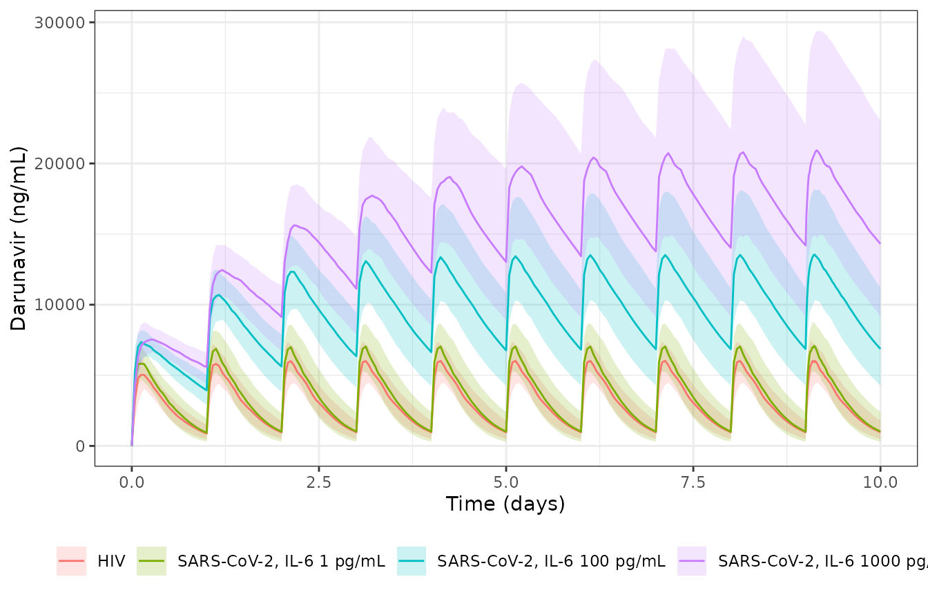
Replicates Figure 4 of Cojutti 2020: median (line) and 25th-75th percentiles (band) of darunavir concentration over a 10-day course of 800 mg once daily.
PKNCA validation
NCA over the tenth dosing interval (216-240 h), per subject, grouped by arm.
nca_conc <- sim |>
  filter(time >= 216, !is.na(Cc)) |>
  mutate(treatment = arm) |>
  select(id, time, Cc = Cc_ngml, treatment)
nca_dose <- bind_rows(ev_hiv, ev_covid) |>
  filter(evid == 1) |>
  mutate(treatment = factor(arm, levels = arms)) |>
  select(id, time, amt, treatment)

conc_obj <- PKNCA::PKNCAconc(nca_conc, Cc ~ time | treatment + id)
dose_obj <- PKNCA::PKNCAdose(nca_dose, amt ~ time | treatment + id)
intervals <- data.frame(start = 216, end = 240, cmin = TRUE, cmax = TRUE, tmax = TRUE, auclast = TRUE)
nca_res <- PKNCA::pk.nca(PKNCA::PKNCAdata(conc_obj, dose_obj, intervals = intervals))
knitr::kable(summary(nca_res))| start | end | treatment | N | auclast | cmax | cmin | tmax |
|---|---|---|---|---|---|---|---|
| 216 | 240 | HIV | 200 | 77400 [46.3] | 6110 [37.6] | 839 [169] | 3.25 [0.500, 9.25] |
| 216 | 240 | SARS-CoV-2, IL-6 1 pg/mL | 200 | 86800 [58.5] | 7290 [35.0] | 762 [330] | 2.75 [0.500, 8.25] |
| 216 | 240 | SARS-CoV-2, IL-6 100 pg/mL | 200 | 250000 [58.2] | 14200 [42.2] | 6400 [103] | 3.00 [0.500, 9.25] |
| 216 | 240 | SARS-CoV-2, IL-6 1000 pg/mL | 200 | 430000 [53.6] | 21300 [44.4] | 13800 [70.4] | 3.75 [0.500, 10.8] |
Comparison against the published simulation
The Results report the median steady-state Cmin and Cmax of the
Figure 4 simulations. The Cmax values are printed with a European
thousands separator (5.425, 7.560, …), which
in ng/mL can only mean 5425, 7560, …; a value of 5.4 ng/mL would be
below the paper’s own trough values.
published <- data.frame(
  treatment = arms,
  cmin = c(826, 1460, 7020, 14140),
  cmax = c(5425, 7560, 13418, 20729)
)
simulated <- as.data.frame(nca_res$result) |>
  mutate(treatment = as.character(treatment)) |>
  filter(PPTESTCD %in% c("cmin", "cmax")) |>
  select(id, treatment, PPTESTCD, PPORRES)
cmp <- nlmixr2lib::ncaComparisonTable(
  simulated = simulated,
  reference = published,
  by = "treatment",
  units = c(cmin = "ng/mL", cmax = "ng/mL"),
  tolerance_pct = 20
)
knitr::kable(cmp)| NCA parameter | treatment | Reference | Simulated | % diff |
|---|---|---|---|---|
| Cmax (ng/mL) | HIV | 5420 | 6620 | +21.9%* |
| Cmax (ng/mL) | SARS-CoV-2, IL-6 1 pg/mL | 7560 | 7390 | -2.2% |
| Cmax (ng/mL) | SARS-CoV-2, IL-6 100 pg/mL | 13400 | 13700 | +2.4% |
| Cmax (ng/mL) | SARS-CoV-2, IL-6 1000 pg/mL | 20700 | 21000 | +1.5% |
| Cmin (ng/mL) | HIV | 826 | 966 | +17.0% |
| Cmin (ng/mL) | SARS-CoV-2, IL-6 1 pg/mL | 1460 | 1020 | -30.2%* |
| Cmin (ng/mL) | SARS-CoV-2, IL-6 100 pg/mL | 7020 | 6860 | -2.2% |
| Cmin (ng/mL) | SARS-CoV-2, IL-6 1000 pg/mL | 14100 | 14200 | +0.4% |
med_sim <- simulated |>
  group_by(treatment, PPTESTCD) |>
  summarise(sim = median(PPORRES), .groups = "drop") |>
  left_join(
    tidyr::pivot_longer(published, c(cmin, cmax), names_to = "PPTESTCD", values_to = "pub"),
    by = c("treatment", "PPTESTCD")
  ) |>
  mutate(pct_diff = 100 * (sim - pub) / pub)
cmin_covid <- dplyr::filter(med_sim, PPTESTCD == "cmin")
stopifnot(
  # Centre: across the 8 published medians the typical discrepancy is small.
  abs(median(med_sim$pct_diff)) < 15,
  # The high-IL-6 arms, whose exposure is set by CL/F and Vd rather than by
  # the absorption tail, reproduce the published trough and peak.
  all(abs(med_sim$pct_diff[med_sim$treatment %in% arms[3:4]]) < 15),
  # The IL-6 ordering the paper reports is reproduced.
  all(diff(cmin_covid$sim[match(arms[2:4], cmin_covid$treatment)]) > 0)
)
The largest differences are the HIV peak and the SARS-CoV-2 trough at
IL-6 = 1 pg/mL (both flagged above), in the two low-exposure arms. The
low-IL-6 trough depends strongly on the lower tail of ka
(omega 0.82) and on the draw, and the published numbers are themselves a
Monte Carlo estimate from Mlxplore. The HIV peak is high even without
variability: the typical-value steady-state Cmax from Table 2 (CL/F 10.3
L/h, Vd 96.9 L, ka 0.58 1/h) is about 6200 ng/mL against the published
5425 ng/mL, so the gap is not a sampling artefact; the paper does not
say how its simulated Cmax was summarised (for instance per subject, or
as the peak of the median profile, which is about 6000 ng/mL here). The
high-IL-6 arms, whose exposure is set by CL/F and Vd, agree within a few
percent. Nothing was adjusted to close the gap.
As an additional orientation (not gated), the typical steady-state AUC over a dosing interval is Dose / (CL/F): 7.767^{4} ngh/mL for HIV and 1.95122^{5} ngh/mL for a SARS-CoV-2 patient at IL-6 = 31 pg/mL, against the paper’s median individual AUCs of 75,727 and 161,387 ng*h/mL (Results 3.1).
Assumptions and deviations
- IL-6 and BSA centring. The paper prints the covariate exponents but not the centring values. Both covariates are centred on the SARS-CoV-2 cohort medians from Table 1 (IL-6 31 pg/mL, BSA 1.86 m^2). The IL-6 choice is checked against the paper’s Figure 4 simulations above; the BSA choice has no independent check (Figure 4 does not vary BSA) and BSA is the same in both cohorts.
-
Between-subject variability. Table 2 labels the
omega rows
(%), but the values (0.13-1.14) are Monolix standard deviations of the log-scale random effect; a 0.53% CV would be negligible. They are encoded as variances (omega^2). No correlations between random effects were reported, so the omega matrices are diagonal. -
Table 2 bootstrap medians. For the SARS-CoV-2 ka
and Vd the bootstrap median (0.58 1/h, 77.81 L) differs from the point
estimate and lies near or outside its own 99% CI; the point estimates in
the
Valuecolumn are used. - IL-6 as time-fixed. IL-6 was measured on the TDM day and entered as one value per patient; the model accepts a time-varying IL-6 column, but the source did not estimate such a use.
- Booster. SARS-CoV-2 patients received cobicistat- or ritonavir-boosted darunavir (73% cobicistat); the model does not distinguish them, in line with the bioequivalence cited in Methods 2.1.
-
Figure 4 Cmax separator. The Results print the
simulated Cmax values as
5.425,7.560,13.418and20.729ng/mL; these are read as thousands (5425 ng/mL, …). - Units. The model files work in mg and L (concentration mg/L); the paper reports ng/mL. The vignette multiplies by 1000 for comparison.