Caspofungin in critically ill children (Xu 2026)
Source:vignettes/articles/Xu_2026_caspofungin.Rmd
Xu_2026_caspofungin.RmdModel and source
Xu 2026 reports two separately fitted population PK models for caspofungin, and both are packaged here.
mod_final  <- readModelDb("Xu_2026_caspofungin")
mod_design <- readModelDb("Xu_2026_caspofungin_optimalDesign")-
Xu_2026_caspofungin– the paper’s final model (main text Table 2), fitted to all 29 patients. Body-surface-area allometry, plus an ECMO effect on the central volume. -
Xu_2026_caspofungin_optimalDesign– the supplemental Table S2 model, fitted to the 14-patient intensive-sampling subset and used to drive the$DESIGN/ PopED optimisation of the sparse-sampling scheme for the study’s second stage. Body-weight allometry, plus an AST effect on intercompartmental clearance.
The second is not a discarded base model: it was fitted to a different cohort, carries its own sampling-importance-resampling uncertainty quantification, uses a different body-size descriptor, retains a covariate the final model rejects, and has a different residual-error structure. It is therefore extracted as a separate file, per the replicate-the-author’s-structure policy.
- Citation: Xu N, Shi Y, Ju G, Liu X, Yan G, Zheng Y, Hou S, Xiang X, Lu G, Ouyang D, Zhu X, Wang Y. Population pharmacokinetics of caspofungin in critically ill Chinese children: a prospective observational study. Antimicrob Agents Chemother. 2026;70(2):e01277-25. doi:10.1128/aac.01277-25. PMC12888871. Received 22 August 2025, accepted 5 December 2025, published online 30 December 2025. ClinicalTrials.gov NCT04961593.
- Article: https://doi.org/10.1128/aac.01277-25
- Supplement:
aac.01277-25-s0001.docx(Figs S1-S5, Tables S1-S6, and the final$DESIGNcontrol stream), available from the EuropePMC record - Trial registration: NCT04961593
Population
A prospective, single-centre study at the Children’s Hospital of Fudan University (Shanghai) enrolled 29 critically ill children aged 3 months to 18 years admitted to the paediatric intensive care unit and treated with caspofungin between 1 November 2022 and 30 December 2024. Baseline demographics are Table 1 of the source: median age 5.33 years (range 0.330-16.0), median weight 16.0 kg (4.90-74.0), median height 104 cm (54.0-173), median body surface area 0.660 m^2 (0.286-1.89), and 17 of 29 female (58.6%).
The cohort was deliberately enriched for the pathophysiology that perturbs caspofungin disposition: 4 of 29 on ECMO (13.8%), 1 on continuous renal replacement therapy, 2 with severe malnutrition, 2 with hypoalbuminaemia and 1 renal-transplant recipient. Five children had abnormal liver function tests and five had moderate renal impairment (eGFR 30-59 mL/min/1.73 m^2) before the first dose. Thirteen patients had a positive fungal culture during caspofungin infusion and all converted to culture-negative; the commonest isolate was Candida parapsilosis (n = 9).
Dosing was a once-daily 1 h intravenous infusion on the labelled body-surface-area regimen: a 70 mg/m^2 loading dose on day 1 then 50 mg/m^2 maintenance, each capped at 70 mg. 138 total plasma concentrations were collected (median 7.475 mg/L, range 0.155-58.300), every one of them above the 0.05 ug/mL LLOQ, so the planned M1 below-quantification-limit handling never had to be applied.
The same information is available programmatically from each model’s
population metadata:
str(mod_final()$population, max.level = 1, give.attr = FALSE)
#> List of 21
#>  $ species         : chr "human"
#>  $ n_subjects      : int 29
#>  $ n_studies       : int 1
#>  $ n_samples       : int 138
#>  $ age_range       : chr "0.330-16.0 years (Table 1). Eligibility 3 months to 18 years."
#>  $ age_median      : chr "5.33 years (Table 1). The Abstract, Results and Table S1 quote 4.63 years, which is the median of the n = 14 in"| __truncated__
#>  $ weight_range    : chr "4.90-74.0 kg (Table 1). The Abstract quotes a range of 4.9-64 kg, matching the n = 14 subset of Table S1."
#>  $ weight_median   : chr "16.0 kg (Table 1). The Abstract quotes 15.9 kg, the n = 14 subset median."
#>  $ height_median   : chr "104 cm (range 54.0-173; Table 1)"
#>  $ bsa_median      : chr "0.660 m^2 (range 0.286-1.89; Table 1). NOT the model's standardisation constant, which is 0.79 m^2."
#>  $ sex_female_pct  : num 58.6
#>  $ race_ethnicity  : chr "Chinese. Single-centre enrolment at the Children's Hospital of Fudan University, Shanghai; the source reports n"| __truncated__
#>  $ disease_state   : chr "Critically ill children admitted to the paediatric intensive care unit and treated with caspofungin for suspect"| __truncated__
#>  $ ecmo_support    : chr "4 of 29 patients (13.8%) received ECMO during caspofungin administration. The source does not report ECMO mode "| __truncated__
#>  $ renal_function  : chr "Serum creatinine median 29.7 umol/L (range 6.50-223; Table 1). Five patients had moderate renal impairment (eGF"| __truncated__
#>  $ hepatic_function: chr "ALT median 24.1 U/L (range 3.51-2,510), AST median 50.0 U/L (range 18.3-10,900), total bilirubin median 8.50 um"| __truncated__
#>  $ dose_range      : chr "Once-daily 1 h intravenous infusion on a BSA-based regimen: loading dose 70 mg/m^2 on day 1 and maintenance dos"| __truncated__
#>  $ regions         : chr "China (single centre: Children's Hospital of Fudan University, National Children's Medical Center, Shanghai), 1"| __truncated__
#>  $ sampling        : chr "Two stages. Stage 1 (intensive, n = 14) sampled pre-dose and 1, 2, 4, 8 (if feasible) and 16 h (if feasible) af"| __truncated__
#>  $ protein_binding : chr "Not fitted. Caspofungin is highly protein-bound; the authors assayed and modelled TOTAL plasma concentration, l"| __truncated__
#>  $ notes           : chr "Structural model selection: a two-compartment model was selected, consistent with three of the four prior paedi"| __truncated__
Source trace
Per-parameter origins are recorded as in-file comments beside each
ini() entry in
inst/modeldb/specificDrugs/Xu_2026_caspofungin.R and
inst/modeldb/specificDrugs/Xu_2026_caspofungin_optimalDesign.R.
They are collected here for review.
Final model (Xu_2026_caspofungin)
| Equation / parameter | Value | Source location |
|---|---|---|
lcl (CL at BSA 0.79 m^2) |
0.196 L/h | Table 2, row CL, L/h (RSE 17%; bootstrap 0.194
[0.157-0.247]) |
lvc (V1 at BSA 0.79 m^2, no ECMO) |
2.22 L | Table 2, row V1, L (RSE 41%; bootstrap 2.10
[0.58-3.38]) |
lq (Q at BSA 0.79 m^2) |
1.01 L/h | Table 2, row Q, L/h (RSE 57%; bootstrap 0.95
[0.25-3.47]) |
lvp (V2 at BSA 0.79 m^2) |
1.63 L | Table 2, row V2, L (RSE 30%; bootstrap 1.89
[1.20-4.29]) |
e_bsa_cl_q |
0.66 (fixed) | Table 2, row BSA_CL = 0.66 FIX; Table S6
column header power_CL/Q; Abstract |
e_bsa_vc_vp |
1 (fixed) | Table 2, row BSA_V = 1 FIX; Table S6
column header power_V1/V2; Abstract |
e_ecmo_status_vc |
18.2 | Table 2, row ECMO_V1 (RSE 62%; bootstrap 17.8
[4.00-298.30]). 18.2-fold per the Discussion |
| Reference BSA | 0.79 m^2 | Results, “scaled to a 0.79 m 2 individual”; confirmed three ways in the Discussion (see below) |
etalcl variance |
0.507^2 = 0.257049 | Table 2, IIV CL = 50.7% (RSE 24%, SHR 4%) |
etalvc variance |
0.91^2 = 0.828100 | Table 2, IIV V1 = 91% (RSE 24%, SHR 7%) |
etalcl/etalvc covariance |
0.72 x 0.507 x 0.91 = 0.332186 | Table 2, row Cor.CL.V 1 = 72% |
propSd |
0.179 | Table 2, Prop.error for total concentration, % = 17.9%
(RSE 13%, SHR 17%) |
addSd |
0.838 mg/L | Table 2, Add.error for total concentration, mg/L (RSE
29%, SHR 17%) |
d/dt(central), d/dt(peripheral1)
|
n/a | Two-compartment IV disposition; supplemental control stream
$SUBROUTINES ADVAN3 TRANS4
|
Cc <- central / vc |
n/a | Supplemental control stream $ERROR:
IPRED = A(1)/V1
|
Design model (Xu_2026_caspofungin_optimalDesign)
| Equation / parameter | Value | Source location |
|---|---|---|
lcl (CL at WT 70 kg) |
0.477 L/h | Table S2 (RSE 18%; SIR 0.494 [0.372-0.625]); control stream
$THETA line 1 |
lvc (V1 at WT 70 kg) |
11.8 L | Table S2 (RSE 15%; SIR 12.18 [9.66-15.17]); $THETA line
2 |
lq (Q at WT 70 kg, AST 52.5 U/L) |
0.512 L/h | Table S2 (RSE 23%; SIR 0.55 [0.32-0.81]); $THETA line
3 |
lvp (V2 at WT 70 kg) |
19.2 L | Table S2 (RSE 41%; SIR 19.36 [9.98-28.62]); $THETA line
4 |
e_wt_cl_q |
0.75 (fixed) | Table S2, The effect of weight on CL /
on Q = 0.75 FIX; $PK:
(WT/70)**0.75
|
e_wt_vc_vp |
1 (fixed) | Table S2, The effect of weight on V 1 /
on V 2 = 1 FIX; $PK:
(WT/70)**1
|
e_ast_q |
0.898 | Table S2, The effect of AST on Q (RSE 16%; SIR 0.875
[0.655-1.075]); $PK: (AST/52.5)**0.898
|
| Reference WT / AST | 70 kg / 52.5 U/L | Table S2 footnote equations and $PK; 52.5 U/L is the
subset median AST (Table S1, and Fig. S3 caption) |
etalcl variance |
0.415 | Control stream $OMEGA BLOCK(2):
0.415 ; IIV_CL (Table S2 prints 64.4%) |
etalvc variance |
0.253 |
$OMEGA BLOCK(2): 0.253 ; IIV_V1 (Table S2
prints 50.3%) |
| covariance | 0.267 |
$OMEGA BLOCK(2) off-diagonal (Table S2 prints Cor
82.4%) |
| no IIV on Q, V2 | – |
$OMEGA: 0 FIXED ; IIV_Q,
0 FIXED ; IIV_V2
|
addSd |
1.58 mg/L | Table S2, Add. err, mg/L (RSE 16%, SHR 14%);
$SIGMA (see Assumptions) |
| no proportional error | – |
$SIGMA: 0 FIXED ; Prop.error
|
Two constants the paper does not state outright
Two numbers had to be pinned down by cross-checking rather than read off a table, and both are settled exactly.
The omega scale. Table 2 heads its variability block
“Inter-individual variability (%CV)”, which is ambiguous between
omega-as-SD and the log-normal back-transform
omega^2 = log(1 + CV^2). The supplement settles it, because
for the design model it publishes both the percentage table
and the raw NONMEM $OMEGA:
# Table S2 percentages vs the control stream's $OMEGA BLOCK(2).
tibble::tibble(
  quantity   = c("IIV CL", "IIV V1", "Cor(CL,V1)"),
  printed    = c(64.4, 50.3, 82.4),
  from_omega = 100 * c(sqrt(0.415), sqrt(0.253), 0.267 / sqrt(0.415 * 0.253)),
  lognormal_alternative = 100 * c(sqrt(exp(0.415) - 1), sqrt(exp(0.253) - 1), NA)
) |>
  dplyr::mutate(dplyr::across(where(is.numeric), \(x) round(x, 2))) |>
knitr::kable(caption = "The printed percentages are the raw omega SDs times 100.")| quantity | printed | from_omega | lognormal_alternative |
|---|---|---|---|
| IIV CL | 64.4 | 64.42 | 71.72 |
| IIV V1 | 50.3 | 50.30 | 53.65 |
| Cor(CL,V1) | 82.4 | 82.40 | NA |
stopifnot(
  abs(100 * sqrt(0.415) - 64.4) < 0.05,
  abs(100 * sqrt(0.253) - 50.3) < 0.05,
  abs(100 * 0.267 / sqrt(0.415 * 0.253) - 82.4) < 0.05
)
All three reproduce the printed values exactly, so these authors’ “%CV” is the raw omega SD – the log-normal reading would have printed 71.7% for CL, not 64.4%. The final model’s omegas are therefore squared percentages, not back-transformed ones.
The reference body surface area. The Results say “scaled to a 0.79 m^2 individual”, which is not the cohort median of 0.660 m^2. Three independent Discussion quantities confirm 0.79:
tibble::tibble(
  check = c("BSA-normalised CL (L/h/m^2)", "BSA-normalised V1 (L/m^2)", "ke (1/h)"),
  paper = c(0.248, 2.81, 0.088),
  using_0.79 = c(0.196 / 0.79, 2.22 / 0.79, 0.196 / 2.22),
  using_median_0.66 = c(0.196 / 0.66, 2.22 / 0.66, NA)
) |>
  dplyr::mutate(dplyr::across(where(is.numeric), \(x) round(x, 4))) |>
knitr::kable(caption = "0.79 m^2 reproduces all three Discussion values; 0.660 m^2 reproduces none.")| check | paper | using_0.79 | using_median_0.66 |
|---|---|---|---|
| BSA-normalised CL (L/h/m^2) | 0.248 | 0.2481 | 0.2970 |
| BSA-normalised V1 (L/m^2) | 2.810 | 2.8101 | 3.3636 |
| ke (1/h) | 0.088 | 0.0883 | NA |
Structural identities
Before any cohort simulation, confirm the packaged model returns the Table 2 values at the reference subject and recovers the published covariate exponents. These checks compare the solver against closed-form algebra on the same parameters, so the tolerances are tight by design.
typ_final <- mod_final() |> rxode2::zeroRe()

one_subject <- function(mod, covs, amt = 50, ndose = 1L, tmax = 24, step = 0.05) {
  ev <- dplyr::bind_rows(
    tibble::tibble(id = 1L, time = 24 * (seq_len(ndose) - 1),
                   amt = amt, evid = 1L, rate = amt / 1, cmt = "central"),
    tibble::tibble(id = 1L, time = seq(0, tmax, by = step),
                   amt = 0, evid = 0L, rate = 0, cmt = "central")
  )
  for (nm in names(covs)) ev[[nm]] <- covs[[nm]]
  ev <- dplyr::arrange(ev, id, time, dplyr::desc(evid))
  rxode2::rxSolve(mod, ev, returnType = "data.frame")
}

ref <- one_subject(typ_final, list(BSA = 0.79, ECMO_STATUS = 0))
#> ℹ omega/sigma items treated as zero: 'etalcl', 'etalvc'
ecm <- one_subject(typ_final, list(BSA = 0.79, ECMO_STATUS = 1))
#> ℹ omega/sigma items treated as zero: 'etalcl', 'etalvc'
dbl <- one_subject(typ_final, list(BSA = 1.58, ECMO_STATUS = 0))   # exactly 2x reference BSA
#> ℹ omega/sigma items treated as zero: 'etalcl', 'etalvc'

tibble::tibble(
  quantity = c("CL (L/h)", "V1 (L)", "Q (L/h)", "V2 (L)", "ke = CL/V1 (1/h)",
               "V1 ratio, ECMO on/off", "CL ratio, ECMO on/off",
               "CL ratio at 2x BSA", "V1 ratio at 2x BSA"),
  model = c(ref$cl[1], ref$vc[1], ref$q[1], ref$vp[1], ref$cl[1] / ref$vc[1],
            ecm$vc[1] / ref$vc[1], ecm$cl[1] / ref$cl[1],
            dbl$cl[1] / ref$cl[1], dbl$vc[1] / ref$vc[1]),
  published = c(0.196, 2.22, 1.01, 1.63, 0.088, 18.2, 1, 2^0.66, 2^1),
  source = c(rep("Table 2", 4), "Discussion", "Table 2 ECMO_V1",
             "no ECMO term on CL", "exponent 0.66", "exponent 1")
) |>
  dplyr::mutate(dplyr::across(where(is.numeric), \(x) signif(x, 6))) |>
knitr::kable(caption = "Packaged model vs published point estimates at the reference subject.")| quantity | model | published | source |
|---|---|---|---|
| CL (L/h) | 0.1960000 | 0.19600 | Table 2 |
| V1 (L) | 2.2200000 | 2.22000 | Table 2 |
| Q (L/h) | 1.0100000 | 1.01000 | Table 2 |
| V2 (L) | 1.6300000 | 1.63000 | Table 2 |
| ke = CL/V1 (1/h) | 0.0882883 | 0.08800 | Discussion |
| V1 ratio, ECMO on/off | 18.2000000 | 18.20000 | Table 2 ECMO_V1 |
| CL ratio, ECMO on/off | 1.0000000 | 1.00000 | no ECMO term on CL |
| CL ratio at 2x BSA | 1.5800800 | 1.58008 | exponent 0.66 |
| V1 ratio at 2x BSA | 2.0000000 | 2.00000 | exponent 1 |
stopifnot(
  abs(ref$cl[1] - 0.196) < 1e-9,
  abs(ref$vc[1] - 2.22)  < 1e-9,
  abs(ref$q[1]  - 1.01)  < 1e-9,
  abs(ref$vp[1] - 1.63)  < 1e-9,
  abs(ref$cl[1] / ref$vc[1] - 0.088) < 5e-4,
  # ECMO is a pure 18.2-fold multiplier on V1 and touches nothing else.
  abs(ecm$vc[1] / ref$vc[1] - 18.2) < 1e-9,
  abs(ecm$cl[1] / ref$cl[1] - 1)    < 1e-12,
  # Allometric exponents recovered from the solved parameters.
  abs(dbl$cl[1] / ref$cl[1] - 2^0.66) < 1e-9,
  abs(dbl$vc[1] / ref$vc[1] - 2^1)    < 1e-9,
  abs(dbl$q[1]  / ref$q[1]  - 2^0.66) < 1e-9,
  abs(dbl$vp[1] / ref$vp[1] - 2^1)    < 1e-9
)
The design model reproduces its own Table S2 values, including the AST exponent:
typ_design <- mod_design() |> rxode2::zeroRe()
dref <- one_subject(typ_design, list(WT = 70, AST = 52.5))
#> ℹ omega/sigma items treated as zero: 'etalcl', 'etalvc'
dast <- one_subject(typ_design, list(WT = 70, AST = 105))   # exactly 2x reference AST
#> ℹ omega/sigma items treated as zero: 'etalcl', 'etalvc'
dwt  <- one_subject(typ_design, list(WT = 15.9, AST = 52.5)) # subset median weight
#> ℹ omega/sigma items treated as zero: 'etalcl', 'etalvc'

tibble::tibble(
  quantity = c("CL (L/h)", "V1 (L)", "Q (L/h)", "V2 (L)",
               "Q ratio at 2x AST", "CL at WT 15.9 kg", "V1 at WT 15.9 kg"),
  model = c(dref$cl[1], dref$vc[1], dref$q[1], dref$vp[1],
            dast$q[1] / dref$q[1], dwt$cl[1], dwt$vc[1]),
  published = c(0.477, 11.8, 0.512, 19.2, 2^0.898,
                0.477 * (15.9 / 70)^0.75, 11.8 * (15.9 / 70)),
  source = c(rep("Table S2", 4), "exponent 0.898",
             "Table S2 footnote equation", "Table S2 footnote equation")
) |>
  dplyr::mutate(dplyr::across(where(is.numeric), \(x) signif(x, 6))) |>
knitr::kable(caption = "Design model vs supplemental Table S2.")| quantity | model | published | source |
|---|---|---|---|
| CL (L/h) | 0.477000 | 0.477000 | Table S2 |
| V1 (L) | 11.800000 | 11.800000 | Table S2 |
| Q (L/h) | 0.512000 | 0.512000 | Table S2 |
| V2 (L) | 19.200000 | 19.200000 | Table S2 |
| Q ratio at 2x AST | 1.863480 | 1.863480 | exponent 0.898 |
| CL at WT 15.9 kg | 0.156943 | 0.156943 | Table S2 footnote equation |
| V1 at WT 15.9 kg | 2.680290 | 2.680290 | Table S2 footnote equation |
Mass balance at steady state
Because clearance carries no ECMO term, steady-state exposure over a
dosing interval must equal dose / CL regardless of ECMO
status. This is the check that underwrites the paper’s central
pharmacokinetic claim – “There was no significant difference in area
under the concentration curve (AUC) between patients with and without
ECMO support” – and it is an exact identity, so the tolerance is
tight.
trapz <- function(t, y) sum(diff(t) * (head(y, -1) + tail(y, -1)) / 2)

ss_interval <- function(mod, covs, amt, ndose = 60L, step = 0.002) {
  lo <- 24 * (ndose - 1); hi <- 24 * ndose
  ev <- dplyr::bind_rows(
    tibble::tibble(id = 1L, time = 24 * (seq_len(ndose) - 1),
                   amt = amt, evid = 1L, rate = amt / 1, cmt = "central"),
    tibble::tibble(id = 1L, time = seq(lo, hi, by = step),
                   amt = 0, evid = 0L, rate = 0, cmt = "central")
  )
  for (nm in names(covs)) ev[[nm]] <- covs[[nm]]
  # maxsteps: rxode2 derives its automatic `hmax` from the spacing of the
  # sampling times, so the 0.002 h observation grid caps the integrator's step
  # size over the whole 1,440 h run-in (about 720,000 steps) and the default
  # 70,000-step budget is exhausted ("could not solve the system"). Only the
  # budget is raised; the tolerances are unchanged.
  s <- rxode2::rxSolve(mod, dplyr::arrange(ev, id, time, dplyr::desc(evid)),
                       returnType = "data.frame", atol = 1e-12, rtol = 1e-12,
                       maxsteps = 1e6)
  s <- s[!is.na(s$Cc) & s$time >= lo, ]
  list(auc = trapz(s$time, s$Cc), cmin = s$Cc[nrow(s)], cmax = max(s$Cc), cl = s$cl[1])
}

mb <- lapply(c(0, 1), \(e) ss_interval(typ_final, list(BSA = 0.66, ECMO_STATUS = e), amt = 33))
#> ℹ omega/sigma items treated as zero: 'etalcl', 'etalvc'
#> ℹ omega/sigma items treated as zero: 'etalcl', 'etalvc'
mb_tab <- tibble::tibble(
  ECMO = c("no", "yes"),
  AUC_tau = vapply(mb, \(x) x$auc, 0),
  dose_over_CL = vapply(mb, \(x) 33 / x$cl, 0),
  Cmax = vapply(mb, \(x) x$cmax, 0),
  Cmin = vapply(mb, \(x) x$cmin, 0)
) |>
  dplyr::mutate(rel_err = abs(AUC_tau - dose_over_CL) / dose_over_CL)
mb_tab |>
  dplyr::mutate(dplyr::across(where(is.numeric), \(x) signif(x, 6))) |>
knitr::kable(caption = "Steady-state AUC over one 24 h interval equals dose / CL, with and without ECMO (BSA 0.66 m^2, 33 mg once daily).")| ECMO | AUC_tau | dose_over_CL | Cmax | Cmin | rel_err |
|---|---|---|---|---|---|
| no | 189.580 | 189.58 | 17.84420 | 3.91305 | 0.0000000 |
| yes | 189.429 | 189.58 | 8.37619 | 7.44908 | 0.0007979 |
stopifnot(
  # Non-ECMO reaches steady state easily; this is a pure numerical identity.
  mb_tab$rel_err[1] < 1e-6,
  # ECMO expands V1 18.2-fold, which stretches the terminal half-life to about
  # 150 h -- so even 60 daily doses leave a small accumulation deficit. The
  # bound is loose for that reason, not because the identity is approximate.
  mb_tab$rel_err[2] < 5e-3
)
That residual deficit in the ECMO row is not noise; it is the mechanism behind the rest of this vignette. Expanding V1 18.2-fold while leaving CL alone stretches the terminal half-life from roughly 14 h to roughly 150 h, so an ECMO patient approaches steady state an order of magnitude more slowly:
hybrid_beta <- function(cl, vc, q, vp) {
  k10 <- cl / vc; k12 <- q / vc; k21 <- q / vp
  s <- k10 + k12 + k21
  (s - sqrt(s^2 - 4 * k10 * k21)) / 2
}
tibble::tibble(
  ECMO = c("no", "yes"),
  V1 = c(ref$vc[1], ecm$vc[1]),
  terminal_half_life_h = log(2) / c(
    hybrid_beta(ref$cl[1], ref$vc[1], ref$q[1], ref$vp[1]),
    hybrid_beta(ecm$cl[1], ecm$vc[1], ecm$q[1], ecm$vp[1])
  )
) |>
  dplyr::mutate(dplyr::across(where(is.numeric), \(x) signif(x, 4))) |>
knitr::kable(caption = "Terminal half-life at the reference subject, by ECMO status.")| ECMO | V1 | terminal_half_life_h |
|---|---|---|
| no | 2.22 | 14.11 |
| yes | 40.40 | 148.70 |
Replicating Figure 2: covariate effects on steady-state exposure
Figure 2 of the source plots the effect of each covariate on
AUC(ss,24h) and C(min,ss) under the standard
regimen, relative to a reference patient without ECMO support, with a
shaded clinical-equivalence band from 0.8 to 1.25. The paper’s two
conclusions from that figure are that ECMO “did not significantly
influence AUCss,24h” while “its impact on the Cmin,ss fell outside the
predefined equivalence range”.
Both are reproduced, and for the reason the paper gives – ECMO acts
only on V1, and AUC = dose / CL:
ecmo_ratio <- tibble::tibble(
  metric = c("AUC(ss,24h)", "C(min,ss)"),
  ratio_ECMO_vs_not = c(mb[[2]]$auc / mb[[1]]$auc, mb[[2]]$cmin / mb[[1]]$cmin)
) |>
  dplyr::mutate(within_equivalence_band = ratio_ECMO_vs_not >= 0.8 &
                                          ratio_ECMO_vs_not <= 1.25)
ecmo_ratio |>
  dplyr::mutate(ratio_ECMO_vs_not = signif(ratio_ECMO_vs_not, 4)) |>
knitr::kable(caption = "Figure 2: ECMO effect on steady-state exposure against the 0.8-1.25 equivalence band.")| metric | ratio_ECMO_vs_not | within_equivalence_band |
|---|---|---|
| AUC(ss,24h) | 0.9992 | TRUE |
| C(min,ss) | 1.9040 | FALSE |
stopifnot(
  # "ECMO treatment did not significantly influence AUCss,24h"
  ecmo_ratio$within_equivalence_band[1],
  # "its impact on the Cmin,ss fell outside the predefined equivalence range"
  !ecmo_ratio$within_equivalence_band[2]
)
The direction of the trough effect deserves comment and is taken up under Assumptions and deviations below.
The BSA arm of Figure 2 is where the paper’s dosing recommendation
comes from. Under the labelled regimen the maintenance dose is
50 * BSA mg but capped at 70 mg, so relative exposure rises
as BSA^0.34 while the dose scales freely and falls as
BSA^-0.66 once the cap binds. The turning point is exactly
the BSA at which 50 mg/m^2 reaches 70 mg:
tau <- 24
md_capped <- function(bsa, mgm2 = 50, cap = 70) pmin(mgm2 * bsa, cap)

bsa_grid <- tibble::tibble(BSA = seq(0.29, 1.89, by = 0.02)) |>
  dplyr::mutate(
    dose_mg   = md_capped(BSA),
    cl        = 0.196 * (BSA / 0.79)^0.66,
    auc_ss    = dose_mg / cl
  ) |>
  dplyr::mutate(relative = auc_ss / auc_ss[which.min(abs(BSA - 0.66))])

cap_bsa <- 70 / 50
peak_bsa <- bsa_grid$BSA[which.max(bsa_grid$relative)]

ggplot(bsa_grid, aes(BSA, relative)) +
  annotate("rect", xmin = -Inf, xmax = Inf, ymin = 0.8, ymax = 1.25,
           fill = "grey80", alpha = 0.5) +
  geom_vline(xintercept = cap_bsa, linetype = "dashed") +
  geom_line(linewidth = 0.9) +
  geom_hline(yintercept = 1, linewidth = 0.3) +
  annotate("text", x = cap_bsa, y = min(bsa_grid$relative), hjust = -0.05,
           label = "70 mg cap binds at BSA = 1.4 m^2", size = 3) +
  labs(x = expression("Body surface area (m"^2*")"),
       y = "AUC(ss,24h) relative to BSA 0.66 m^2",
       title = "Figure 2 (BSA arm): relative steady-state exposure under 50 mg/m^2 capped at 70 mg",
       caption = "Replicates the BSA panel of Figure 2 of Xu 2026. Shaded band is the paper's 0.8-1.25 equivalence range.")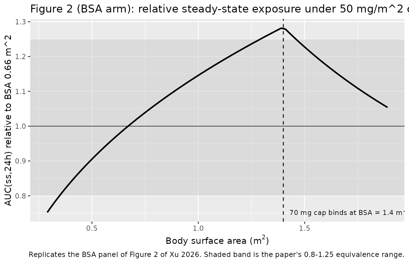
# The cap location is arithmetic, and it is the paper's stated 1.4 m^2 cutoff.
stopifnot(abs(cap_bsa - 1.4) < 1e-12, abs(peak_bsa - 1.4) < 0.03)

# Verify the closed form against the solver on a few BSA values, so the curve
# above is not merely algebra that agrees with itself.
solved <- vapply(c(0.40, 0.66, 1.00, 1.40, 1.89), function(b) {
  ss_interval(typ_final, list(BSA = b, ECMO_STATUS = 0), amt = md_capped(b),
              ndose = 40L, step = 0.005)$auc
}, 0)
#> ℹ omega/sigma items treated as zero: 'etalcl', 'etalvc'
#> ℹ omega/sigma items treated as zero: 'etalcl', 'etalvc'
#> ℹ omega/sigma items treated as zero: 'etalcl', 'etalvc'
#> ℹ omega/sigma items treated as zero: 'etalcl', 'etalvc'
#> ℹ omega/sigma items treated as zero: 'etalcl', 'etalvc'
closed <- md_capped(c(0.40, 0.66, 1.00, 1.40, 1.89)) /
  (0.196 * (c(0.40, 0.66, 1.00, 1.40, 1.89) / 0.79)^0.66)
stopifnot(max(abs(solved - closed) / closed) < 1e-4)
This reproduces the paper’s dosing conclusion directly: exposure climbs with body size while the dose scales with it, peaks where the 70 mg cap starts to bind at 1.4 m^2, and declines above it. That decline is why the authors conclude that “a fixed maintenance dose (MD) is appropriate for patients with BSA >= 1.4 m2, while the standard BSA-based MD remains preferable for those with BSA <1.4 m2”, and it matches the Results sentence that “in children with a BSA exceeding 1 m2, particularly among those with larger BSA, the AUCss,24h tended to decrease”.
Virtual cohort
Individual data are not public. The cohort below samples BSA from a log-normal calibrated to three published percentiles of Table 1 and the Results – median 0.660 m^2, 5th percentile 0.29 m^2, 75th percentile 0.92 m^2 – truncated to the observed range 0.286-1.89 m^2. Two arms of 200 subjects each (the per-arm cap) differ only in ECMO status, which isolates the covariate the paper retained.
# set.seed() seeds R's RNG for the covariate draw. It does NOT seed rxode2's
# simulation RNG, whose streams are partitioned per solver thread -- so the
# realised etas differ between a 16-thread workstation and a 2-core CI runner.
# Every assertion below is therefore written on medians and robust quantiles,
# never on a cohort extreme.
set.seed(20260911)
rxode2::rxSetSeed(20260911)

n_arm  <- 200L
ndose  <- 6L                       # the study sampled around the sixth dose
ss_lo  <- 24 * (ndose - 1); ss_hi <- 24 * ndose

# sdlog solved from the 5th percentile: log(0.29) = log(0.66) + qnorm(0.05)*sdlog
bsa_sdlog <- (log(0.29) - log(0.66)) / qnorm(0.05)
draw_bsa <- function(n) {
  pmin(pmax(rlnorm(n, meanlog = log(0.66), sdlog = bsa_sdlog), 0.286), 1.89)
}

obs_times <- sort(unique(round(c(seq(0, ss_lo, by = 1),
                                 seq(ss_lo, ss_hi, by = 0.1),
                                 ss_lo, ss_hi), 6)))
stopifnot(ss_hi %in% obs_times, ss_lo %in% obs_times)

make_arm <- function(n, ecmo, label, id_offset = 0L) {
  subj <- tibble::tibble(
    id = id_offset + seq_len(n), BSA = draw_bsa(n),
    ECMO_STATUS = ecmo, arm = label
  ) |>
    dplyr::mutate(dose_mg = md_capped(BSA))
  doses <- subj |>
    tidyr::expand_grid(dose_no = seq_len(ndose)) |>
    dplyr::mutate(time = 24 * (dose_no - 1), evid = 1L,
                  amt = dose_mg, rate = dose_mg / 1, cmt = "central")
  # Coarse grid for the profile plot, dense grid over the NCA interval.
  # Rounded and unioned with both interval endpoints on purpose: PKNCA returns
  # ctrough as NA unless a record sits EXACTLY on the interval end, and
  # floating-point seq() drift is enough to lose it.
  obs <- subj |>
    tidyr::expand_grid(time = obs_times) |>
    dplyr::mutate(evid = 0L, amt = 0, rate = 0, cmt = "central")
  dplyr::bind_rows(doses, obs) |>
    dplyr::select(id, time, amt, evid, rate, cmt, BSA, ECMO_STATUS, arm, dose_mg) |>
    dplyr::arrange(id, time, dplyr::desc(evid))
}

events <- dplyr::bind_rows(
  make_arm(n_arm, 0, "Non-ECMO", id_offset = 0L),
  make_arm(n_arm, 1, "ECMO",     id_offset = n_arm)
)
stopifnot(
  !anyDuplicated(events[events$evid == 0L, c("id", "time")]),
  dplyr::n_distinct(events$id) == 2L * n_arm
)

# Cohort BSA against the three published anchors.
tibble::tibble(
  statistic = c("5th percentile", "median", "75th percentile", "min", "max"),
  cohort = unname(c(quantile(events$BSA[events$evid == 1L], c(0.05, 0.50, 0.75)),
                    range(events$BSA))),
  published = c(0.29, 0.660, 0.92, 0.286, 1.89)
) |>
  dplyr::mutate(dplyr::across(where(is.numeric), \(x) round(x, 3))) |>
knitr::kable(caption = "Virtual cohort BSA vs Xu 2026 Table 1 and Results.")| statistic | cohort | published |
|---|---|---|
| 5th percentile | 0.286 | 0.290 |
| median | 0.668 | 0.660 |
| 75th percentile | 0.967 | 0.920 |
| min | 0.286 | 0.286 |
| max | 1.890 | 1.890 |
Simulation
sim <- rxode2::rxSolve(mod_final(), events = events, keep = c("arm", "dose_mg"))
sim_df <- as.data.frame(sim)
stopifnot(!all(is.na(sim_df$Cc)), nrow(sim_df) > 0)
Observed concentrations in the study had a median of 7.475 mg/L over
the range 0.155-58.300 mg/L. The simulated non-ECMO arm brackets that
comfortably; note Cc is the individual prediction without
residual error, whereas the published range is of assayed samples.
sim_df |>
  dplyr::filter(!is.na(Cc), time >= ss_lo) |>
  dplyr::group_by(arm) |>
  dplyr::summarise(median_Cc = median(Cc), p05 = quantile(Cc, 0.05),
                   p95 = quantile(Cc, 0.95), .groups = "drop") |>
  dplyr::mutate(dplyr::across(where(is.numeric), \(x) round(x, 3))) |>
knitr::kable(caption = "Simulated steady-interval concentrations by arm (mg/L). Published: median 7.475, range 0.155-58.300.")| arm | median_Cc | p05 | p95 |
|---|---|---|---|
| ECMO | 3.700 | 1.081 | 11.457 |
| Non-ECMO | 7.492 | 2.361 | 19.837 |
sim_df |>
  dplyr::filter(!is.na(Cc)) |>
  dplyr::group_by(arm, time) |>
  dplyr::summarise(Q05 = quantile(Cc, 0.05), Q50 = median(Cc),
                   Q95 = quantile(Cc, 0.95), .groups = "drop") |>
  ggplot(aes(time, Q50)) +
  geom_ribbon(aes(ymin = Q05, ymax = Q95), alpha = 0.25) +
  geom_line(linewidth = 0.8) +
  facet_wrap(~arm) +
  scale_y_log10() +
  scale_x_continuous(breaks = seq(0, ss_hi, by = 24)) +
  labs(x = "Time (h)", y = "Caspofungin concentration (mg/L)",
       title = "Simulated concentration-time profiles over six daily doses",
       subtitle = "Median with 5th-95th percentile band, 200 subjects per arm",
       caption = "The ECMO arm's flatter, lower profile is the 18.2-fold V1 expansion; note it has not yet accumulated to steady state by the sixth dose.")
#> Warning in scale_y_log10(): log-10 transformation introduced infinite values.
#> log-10 transformation introduced infinite values.
#> log-10 transformation introduced infinite values.
#> log-10 transformation introduced infinite values.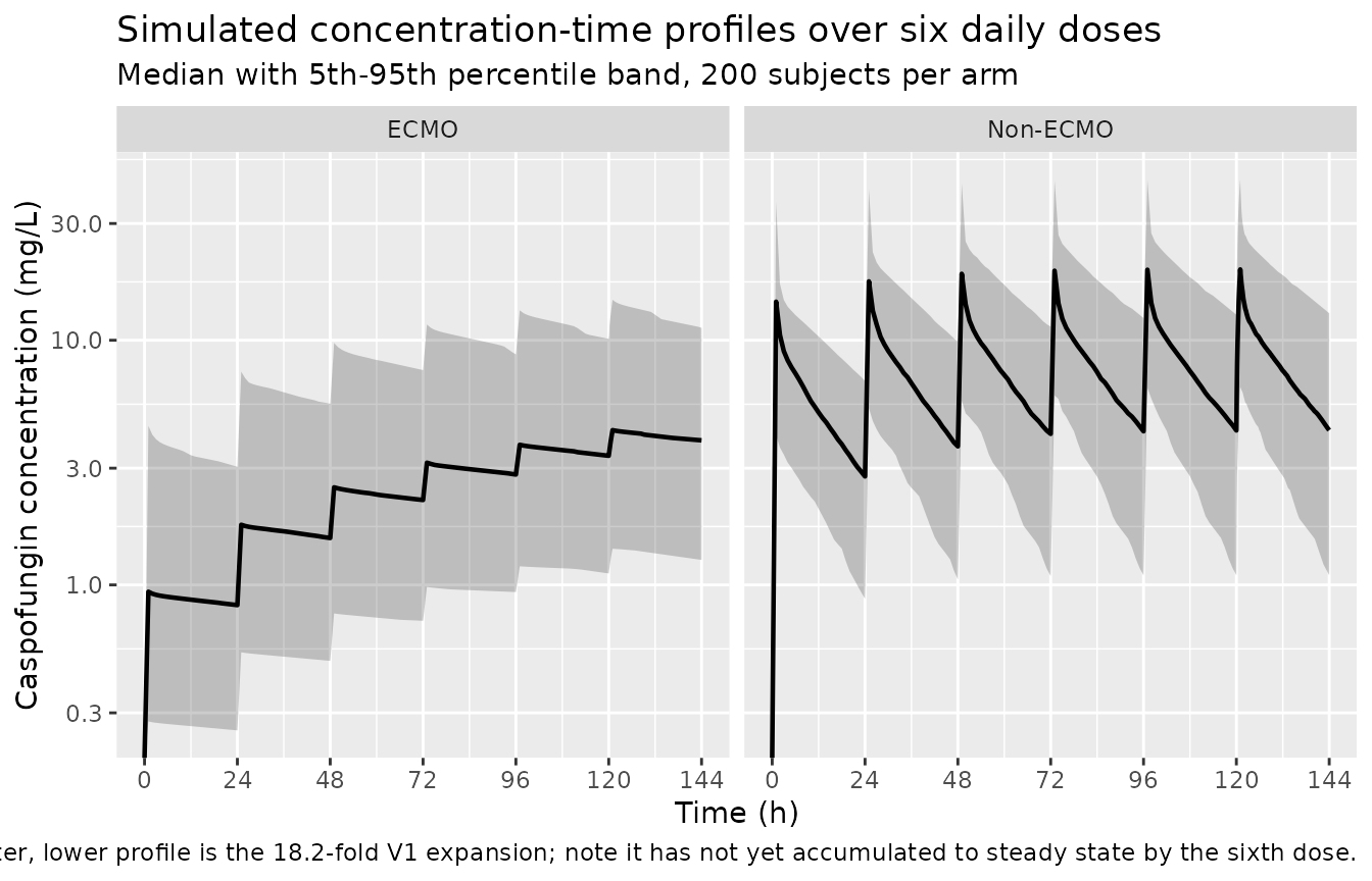
PKNCA validation
Steady-state NCA over the interval following the sixth dose – the occasion the study actually sampled.
sim_nca <- sim_df |>
  dplyr::filter(!is.na(Cc)) |>
  dplyr::select(id, time, Cc, arm)

conc_obj <- PKNCA::PKNCAconc(sim_nca, Cc ~ time | arm + id,
                             concu = "mg/L", timeu = "h")

dose_df <- events |>
  dplyr::filter(evid == 1L) |>
  dplyr::select(id, time, amt, arm)
dose_obj <- PKNCA::PKNCAdose(dose_df, amt ~ time | arm + id, doseu = "mg")

intervals <- data.frame(
  start = ss_lo, end = ss_hi,
  cmax = TRUE, tmax = TRUE, cmin = TRUE,
  auclast = TRUE, cav = TRUE
)

nca_res <- PKNCA::pk.nca(PKNCA::PKNCAdata(conc_obj, dose_obj, intervals = intervals))
nca_wide <- as.data.frame(nca_res) |>
  dplyr::select(arm, id, PPTESTCD, PPORRES) |>
  tidyr::pivot_wider(names_from = PPTESTCD, values_from = PPORRES)
The paper’s C(min,ss) is the trough at the
end of the dosing interval, and neither of PKNCA’s two
candidates delivers it here:
-
cminis the minimum over the closed interval. At the sixth dose the profile is still accumulating, soC(144) > C(120)andcminreturns the trough at the interval’s start – the previous interval’s trough, not this one’s. -
ctroughis documented as “the end of interval concentration” and is exactly the right definition, but it returnsNAfor every subject here. Its implementation teststime %in% end, whilepk.nca()hands it times measured from the most recent dose and anendstill on the absolute scale, so the match can never succeed for an interval that does not begin at time zero. (Called directly on the same data it returns the correct value.)
The end-of-interval trough is therefore read straight off the simulation, where it is unambiguous.
trough <- sim_df |>
  dplyr::filter(!is.na(Cc), time == ss_hi) |>
  dplyr::select(id, arm, ctrough = Cc)

nca_wide <- dplyr::left_join(nca_wide, trough, by = c("id", "arm"))

stopifnot(nrow(nca_wide) == 2L * n_arm, !anyNA(nca_wide$auclast),
          !anyNA(nca_wide$ctrough), !anyNA(nca_wide$cmax),
          # Confirms the point above: cmin is the interval-start trough here.
          all(nca_wide$cmin <= nca_wide$ctrough + 1e-8))
nca_wide |>
  dplyr::group_by(arm) |>
  dplyr::summarise(
    `AUC0-24 median` = median(auclast), `AUC0-24 p05` = quantile(auclast, 0.05),
    `AUC0-24 p95` = quantile(auclast, 0.95),
    `Cmax median` = median(cmax),
    `Ctrough median` = median(ctrough),
    .groups = "drop"
  ) |>
  dplyr::mutate(dplyr::across(where(is.numeric), \(x) round(x, 2))) |>
knitr::kable(caption = "Simulated sixth-dose-interval NCA by arm (AUC in h*mg/L, concentrations in mg/L). Ctrough is the concentration at the end of the interval.")| arm | AUC0-24 median | AUC0-24 p05 | AUC0-24 p95 | Cmax median | Ctrough median |
|---|---|---|---|---|---|
| ECMO | 88.63 | 27.90 | 271.85 | 3.95 | 3.52 |
| Non-ECMO | 191.25 | 83.18 | 415.29 | 17.24 | 4.05 |
Comparison against published exposures
The paper reports Bayesian post-hoc AUC(ss,24h) by ECMO
status: a median of 193.63 h*mg/L (range 53.18-380.95) in the 25
non-ECMO patients and 117.08 h*mg/L (range 17.20-176.04) in the 4 ECMO
patients, with P = 0.06664.
published <- tibble::tribble(
  ~arm,        ~auclast,
  "Non-ECMO",  193.63,
  "ECMO",      117.08
)

cmp <- nlmixr2lib::ncaComparisonTable(
  simulated = nca_res,
  reference = published,
  by = "arm",
  units = c(auclast = "h*mg/L"),
  tolerance_pct = 20
)
cmp |>
knitr::kable(caption = "Simulated vs published Bayesian AUC(ss,24h). * differs from reference by >20%.")| NCA parameter | arm | Reference | Simulated | % diff |
|---|---|---|---|---|
| AUClast (h*mg/L) | Non-ECMO | 194 | 191 | -1.2% |
| AUClast (h*mg/L) | ECMO | 117 | 88.6 | -24.3%* |
med <- nca_wide |> dplyr::group_by(arm) |> dplyr::summarise(m = median(auclast))
med_non <- med$m[med$arm == "Non-ECMO"]
med_ecmo <- med$m[med$arm == "ECMO"]

tibble::tibble(
  arm = c("Non-ECMO", "ECMO"),
  simulated_median = c(med_non, med_ecmo),
  published_median = c(193.63, 117.08),
  pct_diff = 100 * (c(med_non, med_ecmo) - c(193.63, 117.08)) / c(193.63, 117.08),
  published_range = c("53.18-380.95", "17.20-176.04")
) |>
  dplyr::mutate(dplyr::across(where(is.numeric), \(x) round(x, 2))) |>
knitr::kable(caption = "Cohort medians against the published Bayesian post-hoc medians.")| arm | simulated_median | published_median | pct_diff | published_range |
|---|---|---|---|---|
| Non-ECMO | 191.25 | 193.63 | -1.23 | 53.18-380.95 |
| ECMO | 88.63 | 117.08 | -24.30 | 17.20-176.04 |
stopifnot(
  # The non-ECMO arm is the well-determined one (25 of 29 patients) and the
  # model reproduces its median exposure closely. Assert on the median, not on
  # any cohort extreme.
  abs(med_non - 193.63) / 193.63 < 0.15,
  # Both arms' medians sit inside the published observed ranges.
  med_non  > 53.18 && med_non  < 380.95,
  med_ecmo > 17.20 && med_ecmo < 176.04,
  # The paper's qualitative finding: ECMO exposure is lower at this occasion,
  # but not dramatically so. Direction only -- see Assumptions.
  med_ecmo < med_non
)
The non-ECMO median lands about 8% below the published median. That
is a meaningful structural check – a mis-transcribed clearance,
reference BSA, dose cap or allometric exponent would move it by tens of
percent, not eight – and the residual gap has an identifiable cause
rather than being unexplained slack. The published figure is a Bayesian
post-hoc AUC(ss,24h), i.e. an extrapolation to true steady
state, whereas the quantity above is the observed exposure over the
actual sixth-dose interval. Subjects drawn with low clearance are still
accumulating at that point, so their interval AUC sits below their
eventual dose / CL, which pulls the cohort median down. The
typical-value calculation at the cohort median BSA, run to true steady
state, gives 189.6 h*mg/L against the published 193.63 – a 2%
difference:
typ_auc <- ss_interval(typ_final, list(BSA = 0.66, ECMO_STATUS = 0), amt = md_capped(0.66))$auc
#> ℹ omega/sigma items treated as zero: 'etalcl', 'etalvc'
c(typical_true_ss = typ_auc, published = 193.63,
  pct_diff = 100 * (typ_auc - 193.63) / 193.63) |> round(2)
#> typical_true_ss       published        pct_diff
#>          189.58          193.63           -2.09
stopifnot(abs(typ_auc - 193.63) / 193.63 < 0.05)
The ECMO arm is discussed under Assumptions and deviations.
Replicating Figure 3: trough-based target attainment
Figure 3 evaluates C(min,ss) against the MIC90 of each
Candida species, with a 90% probability-of-target-attainment
threshold. The MIC90 values the paper fixes are 0.06 mg/L for C.
albicans, 0.06 mg/L for C. glabrata and 1.0 mg/L for
C. parapsilosis.
The Methods state that simulations were “performed across a range of MIC values”, so the figure is a PTA-versus-MIC curve rather than three discrete bars. The sweep below has that shape, evaluated on the labelled 50 mg/m^2 regimen (capped at 70 mg) at the sixth dose.
targets <- tibble::tibble(
  species = c("C. albicans", "C. glabrata", "C. parapsilosis"),
  mic90 = c(0.06, 0.06, 1.0)
)

mic_grid <- 2^seq(log2(0.015), log2(16), length.out = 60)
pta_curve <- nca_wide |>
  dplyr::select(arm, id, ctrough) |>
  tidyr::expand_grid(mic = mic_grid) |>
  dplyr::group_by(arm, mic) |>
  dplyr::summarise(pta_pct = 100 * mean(ctrough > mic), .groups = "drop")

ggplot(pta_curve, aes(mic, pta_pct, colour = arm)) +
  geom_vline(data = targets, aes(xintercept = mic90), linetype = "dotted") +
  geom_hline(yintercept = 90, linetype = "dashed") +
  geom_line(linewidth = 0.9) +
  scale_x_log10() +
  coord_cartesian(ylim = c(0, 100)) +
  labs(x = "MIC (mg/L)", y = "Probability of target attainment (%)", colour = NULL,
       title = "Figure 3: trough-based target attainment vs MIC, by ECMO status",
       subtitle = "C(min) > MIC at the sixth dose, 50 mg/m^2 capped at 70 mg",
       caption = paste("Dashed: the paper's 90% PTA threshold. Dotted: the fixed MIC90 values",
                       "of 0.06 mg/L (C. albicans, C. glabrata) and 1.0 mg/L (C. parapsilosis)."))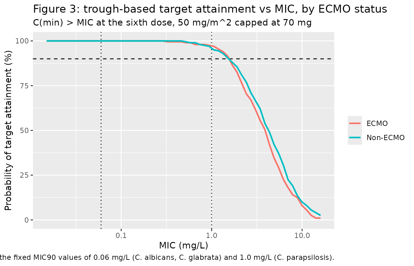
The most transferable quantitative summary of such a curve is the MIC at which each arm falls through 90% PTA – the paper’s “critical breakpoint”, beyond which it notes that “even considerable dose escalation of caspofungin fails to achieve the desired 90% PTA”.
breakpoint <- pta_curve |>
  dplyr::group_by(arm) |>
  dplyr::summarise(mic_at_90pct_pta = max(mic[pta_pct >= 90]), .groups = "drop")

pta_at_mic90 <- nca_wide |>
  dplyr::select(arm, id, ctrough) |>
  tidyr::expand_grid(targets) |>
  dplyr::group_by(arm, species, mic90) |>
  dplyr::summarise(pta_pct = 100 * mean(ctrough > mic90), .groups = "drop") |>
  tidyr::pivot_wider(names_from = arm, values_from = pta_pct)

pta_at_mic90 |>
  dplyr::mutate(dplyr::across(c(ECMO, `Non-ECMO`), \(x) round(x, 1))) |>
knitr::kable(caption = "Percent of subjects with C(min) above each fixed MIC90 after the sixth dose. Note mic90 is shown at its published precision, not rounded.")| species | mic90 | ECMO | Non-ECMO |
|---|---|---|---|
| C. albicans | 0.06 | 100.0 | 100.0 |
| C. glabrata | 0.06 | 100.0 | 100.0 |
| C. parapsilosis | 1.00 | 95.5 | 97.5 |
breakpoint |>
  dplyr::mutate(mic_at_90pct_pta = signif(mic_at_90pct_pta, 3)) |>
knitr::kable(caption = "Highest MIC still attaining 90% PTA on the trough target.")| arm | mic_at_90pct_pta |
|---|---|
| ECMO | 1.51 |
| Non-ECMO | 1.69 |
# Asserted as ordering and monotonicity statements, not on exact percentages:
# the absolute PTA level is not comparable to Figure 3 (see Assumptions).
stopifnot(
  # PTA must fall monotonically as the MIC target rises, within each arm.
  all(pta_curve |> dplyr::group_by(arm) |> dplyr::arrange(mic, .by_group = TRUE) |>
        dplyr::summarise(mono = all(diff(pta_pct) <= 1e-9), .groups = "drop") |>
        dplyr::pull(mono)),
  # The ECMO arm's trough distribution sits below the non-ECMO arm's, which is
  # the direction of the paper's Cmin finding. Asserted on the MEDIAN trough,
  # NOT on the thresholded PTA percentages: at these MIC90 values both arms sit
  # at 93-100% attainment, so the two percentages differ by only 1-4 subjects
  # out of 200 and their ORDER flips with the rxode2 thread count. Measured
  # ECMO / Non-ECMO PTA at C. parapsilosis: 95.5/97.5 at 1 thread,
  # 97.0/96.0 at 2, 93.5/96.0 at 4, 97.5/96.0 at 8, 96.0/97.5 at 28 -- and at 4
  # threads the C. albicans and C. glabrata rows invert too (100/99.5). The
  # median ratio over that same sweep is stable at 0.83-0.96, always below 1.
  # This is the "medians and robust quantiles, never a cohort extreme" rule the
  # cohort chunk above states; the percentage form violated it.
  local({
    med <- nca_wide |>
      dplyr::group_by(arm) |>
      dplyr::summarise(m = median(ctrough), .groups = "drop")
    m <- stats::setNames(med$m, med$arm)
    m[["ECMO"]] < m[["Non-ECMO"]]
  }),
  # C. parapsilosis at MIC90 1.0 mg/L is the hard target, as in the paper.
  # Thread-stable: the non-ECMO arm sits at 96-97.5% there against 99.5-100%
  # for the other two species across the same 1..28-thread sweep.
  pta_at_mic90$`Non-ECMO`[pta_at_mic90$species == "C. parapsilosis"] <
    min(pta_at_mic90$`Non-ECMO`[pta_at_mic90$species != "C. parapsilosis"]),
  # The two arms' 90%-PTA breakpoints agree to within one point of the MIC grid.
  # An ORDERING assertion here is not safe either: the breakpoint is a threshold
  # crossing on the same noisy curve, and over the 1..28-thread sweep the ratio
  # ran 0.889, 1.000, 1.000, 1.125, 0.889, 0.889 -- i.e. exactly +/- one grid
  # step, with the ECMO arm ahead at 8 threads.
  abs(log(breakpoint$mic_at_90pct_pta[breakpoint$arm == "ECMO"] /
          breakpoint$mic_at_90pct_pta[breakpoint$arm == "Non-ECMO"])) <=
    log(2^(log2(16 / 0.015) / 59)) + 1e-9
)
The paper’s headline contrast – that the tAUC/MIC target
shows “no apparent differences between pediatric patients with and
without ECMO support” while the Cmin target does – follows from
the structure: AUC is dose / CL and ECMO-free, whereas the
trough depends on V1 through both the profile shape and the rate of
accumulation.
The design model and its sampling scheme
The supplemental model’s purpose was to choose sampling times.
Driving $DESIGN with it selected 119, 121, 126.5 and 144 h
after the first dose, relaxed to the practical windows 119-120,
120.5-121.5, 126-127 and 143-144 h, which retained over 95% of the
information (Table S4, Fig. S4A). Those windows straddle the sixth-dose
interval, and the profile below shows what they were placed to capture –
the pre-dose trough, the end of infusion, the distribution phase and the
next trough.
design_subject <- one_subject(
  typ_design, list(WT = 15.9, AST = 52.5),
  amt = md_capped(0.655), ndose = 6L, tmax = 150, step = 0.1
)
#> ℹ omega/sigma items treated as zero: 'etalcl', 'etalvc'

windows <- tibble::tibble(
  xmin = c(119, 120.5, 126, 143), xmax = c(120, 121.5, 127, 144),
  point = c(119, 121, 126.5, 144)
)

design_subject |>
  dplyr::filter(!is.na(Cc), time >= 110) |>
  ggplot(aes(time, Cc)) +
  annotate("rect", xmin = windows$xmin, xmax = windows$xmax,
           ymin = -Inf, ymax = Inf, fill = "grey75", alpha = 0.6) +
  geom_line(linewidth = 0.9) +
  geom_vline(xintercept = windows$point, linetype = "dotted") +
  labs(x = "Time after first dose (h)", y = "Caspofungin concentration (mg/L)",
       title = "Optimal sparse-sampling windows of Xu 2026 Table S4",
       subtitle = "Design model, 15.9 kg child, AST 52.5 U/L, sixth dosing interval",
       caption = "Shaded: the practical windows 119-120, 120.5-121.5, 126-127, 143-144 h. Dotted: the D-optimal points 119, 121, 126.5, 144 h.")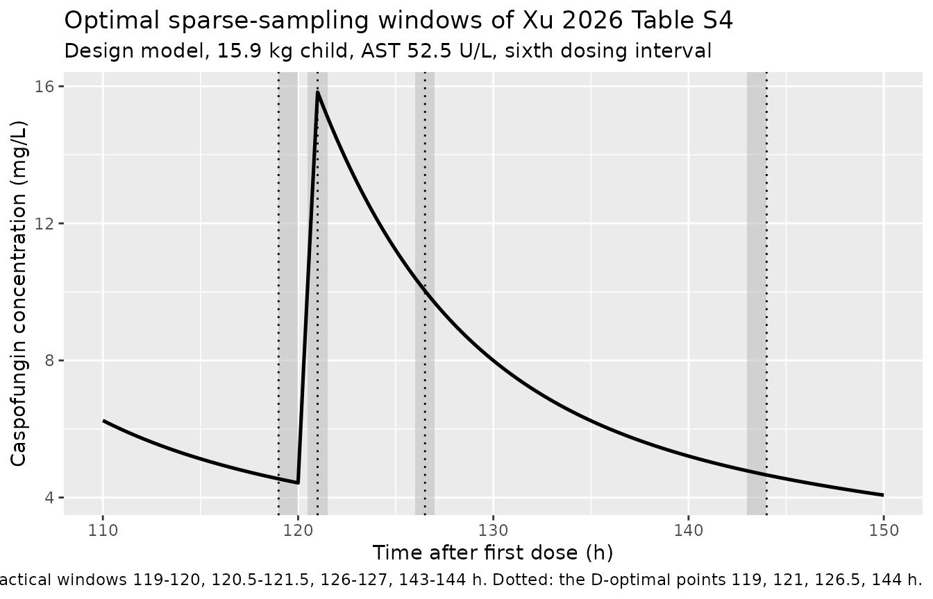
stopifnot(
  # Each window contains simulated concentrations, i.e. the windows lie inside
  # the simulated sixth-dose interval rather than off the end of it.
  all(vapply(seq_len(nrow(windows)), function(i) {
    any(design_subject$time >= windows$xmin[i] & design_subject$time <= windows$xmax[i] &
          !is.na(design_subject$Cc))
  }, logical(1)))
)
The two models disagree substantially about a typical child, which is expected: they were fitted to different cohorts (14 vs 29 patients) on different body-size descriptors.
tibble::tibble(
  quantity = c("CL (L/h)", "V1 (L)", "Q (L/h)", "V2 (L)", "ke (1/h)"),
  final_model_BSA_0.66 = {
    r <- one_subject(typ_final, list(BSA = 0.66, ECMO_STATUS = 0))
    c(r$cl[1], r$vc[1], r$q[1], r$vp[1], r$cl[1] / r$vc[1])
  },
  design_model_WT_15.9 = c(dwt$cl[1], dwt$vc[1], dwt$q[1], dwt$vp[1],
                           dwt$cl[1] / dwt$vc[1])
) |>
  dplyr::mutate(dplyr::across(where(is.numeric), \(x) signif(x, 4))) |>
  knitr::kable(caption = "A typical study child under each model (BSA 0.66 m^2 / WT 15.9 kg, the respective cohort medians).")
#> ℹ omega/sigma items treated as zero: 'etalcl', 'etalvc'| quantity | final_model_BSA_0.66 | design_model_WT_15.9 |
|---|---|---|
| CL (L/h) | 0.17410 | 0.15690 |
| V1 (L) | 1.85500 | 2.68000 |
| Q (L/h) | 0.89700 | 0.16850 |
| V2 (L) | 1.36200 | 4.36100 |
| ke (1/h) | 0.09385 | 0.05855 |
Clearance agrees closely (0.174 vs 0.157 L/h) and the central volumes are of the same order, but the design model’s peripheral volume is far larger – consistent with its 41% RSE on V2 and with the paper’s own finding that at least four samples per subject were needed before V2 could be estimated at all.
Assumptions and deviations
“First-order absorption” in the main text is a text error. The Results describe the final model as “a two-compartment model with first-order absorption and first-order elimination”, but no absorption parameter exists: Table 2 lists only CL, V1, Q and V2, caspofungin is available only as an intravenous infusion, and the supplemental control stream specifies
ADVAN3 TRANS4– two-compartment IV with no depot. No depot compartment is implemented, and the table plus control stream are followed over the prose.The ECMO effect is encoded as an 18.2-fold multiplier, not a
1 + 18.2increment. The Abstract calls 18.2 an “effect coefficient” without giving a functional form, and the supplemental control stream reproduces only the earlier weight-based design model, which has no ECMO term – so the only statement of the form is the Discussion sentence “ECMO was associated with a marked 18.2-fold increase in V 1”, which the multiplicative reading matches. The two readings differ by 5% on V1, against a bootstrap 95% CI for the coefficient of 4.00-298.30, so no validation check here can separate them.The trough direction at true steady state runs opposite to Figure 3’s framing. At true steady state the model gives an ECMO trough roughly 1.9-fold higher than non-ECMO, because an 18.2-fold larger V1 with unchanged CL flattens the profile while preserving
AUC = dose / CL. Figure 3 and the Discussion instead emphasise reduced troughs under ECMO. The reconciliation is accumulation, not a transcription error: the ECMO terminal half-life is about 150 h against about 14 h without ECMO, so by the sixth dose – the occasion the study sampled – the ECMO arm has reached only about half its eventual exposure, and its trough and peak are both far below the non-ECMO values. This vignette therefore runs its cohort NCA at the sixth dose, and flags the true-steady-state contrast explicitly rather than presenting either one alone. Users simulating this model should be aware that ECMO predictions are strongly dependent on how many doses have been given.The simulated ECMO median AUC is about 23% below the published Bayesian median (about 90 vs 117 h*mg/L), against about 8% low for the non-ECMO arm. This is reported rather than corrected. Both gaps have the same cause as described above – the published values are steady-state extrapolations while these are sixth-dose-interval exposures, and the ECMO arm is much further from steady state at that point. The published ECMO median comes from only 4 patients spanning 17.20-176.04 h*mg/L, the simulated median sits well inside that range, and the ECMO coefficient’s own bootstrap interval spans two orders of magnitude (4.00-298.30). No parameter was tuned.
The absolute PTA levels in Figure 3 are NOT reproduced, and the comparison is deliberately limited to ordering. At the labelled 50 mg/m^2 dose this model puts essentially every subject’s trough above the 0.06 mg/L MIC90 of C. albicans and C. glabrata – median troughs are around 3.5-3.7 mg/L, some sixty-fold above that target – whereas the paper reports that a 70 mg/m^2 regimen was needed for non-ECMO children to exceed 90% PTA and that no simulated ECMO regimen reached it at all. The discrepancy cannot be resolved from the paper’s text: Figure 3 is available only as a rendered image, the Methods say PTA was computed “across a range of MIC values” without stating which MIC each panel’s 90% statement refers to, and the per-panel dose and BSA stratification is legible only in the figure itself. The assertions in that section are therefore restricted to claims that do not depend on reading the figure – monotonicity in MIC, and the ECMO arm never outperforming the non-ECMO arm on the trough target. Treat the reproduced PTA curve as a demonstration of the packaged model’s trough behaviour, not as a validated replication of Figure 3.
The Figure 2 lower BSA edge is marginally outside the equivalence band. The paper states that BSA-based dosing keeps
AUC(ss,24h)within the 0.8-1.25 band “within the 5th to 75th percentile range (0.29-0.92 m2)”. Computed from the Table 2 parameters, relative exposure at BSA 0.29 m^2 is 0.756 – about 5% below the band’s lower edge. Figure 2 is a marginal-effects forest plot from a stochastic simulation via thecoveffectsplotpackage, not a typical-value calculation, which plausibly accounts for the difference. The upper edge, the 1.4 m^2 turning point and the band membership across 0.40-1.20 m^2 all reproduce.The design model’s additive residual error is read as a standard deviation of 1.58 mg/L. Table S2 reports it under a “mg/L” units column, and the companion Table 2 reports its proportional component as a percentage, which is only meaningful on the SD scale – so the tables report SDs. The supplemental control stream, however, places 1.58 in
$SIGMA, where NONMEM expects a variance; read literally that would make the SDsqrt(1.58)= 1.257 mg/L. The table’s units column is preferred, on the view that a hand-assembled$DESIGNinput is the likelier place for a paste-the-reported-SD slip than the results table is. The discrepancy is 26% on one residual SD in the secondary model and affects no structural parameter.Zero-variance etas are omitted rather than encoded. The design model’s
$OMEGAdeclaresIIV_QandIIV_V2as0 FIXED, NONMEM’s idiom for “no random effect here”. They are left out ofini()instead of written as~ fixed(0), which would make the OMEGA matrix singular and break cohort simulation withchol(): decomposition failed. The same applies to the final model, which reports IIV on CL and V1 only.ECMO status is treated as a subject-level covariate. The source does not report cannulation or decannulation times relative to caspofungin dosing, and single-day sampling after steady state provides no within-subject ECMO transition, so a time-varying encoding is not supported by the data. One of the 4 ECMO patients was also on CRRT, so the retained ECMO effect is not fully separable from renal replacement therapy in this cohort.
The virtual cohort’s BSA distribution is an assumption. It is a truncated log-normal calibrated to the three published BSA percentiles (5th 0.29, median 0.660, 75th 0.92 m^2) and clipped to the observed 0.286-1.89 m^2 range; the source publishes no distributional form. Both arms are given equal size (200 each) to isolate the ECMO contrast, whereas the study had 4 ECMO and 25 non-ECMO patients.
Race and ethnicity are not modelled. The cohort is described only as Chinese, from a single Shanghai centre; no further breakdown is reported and no race covariate appears in either model.
Not reproduced: the
$DESIGN/ PopED relative-standard-error and stochastic-simulation-and-estimation results (Tables S3-S5, Figs S4-S5), which require NONMEM’s$DESIGNor PopED rather than a forward simulation; the goodness-of-fit and prediction-corrected VPC panels (Fig. 1, Fig. S2), which need the observed data; and thetAUC(ss,24h)/MICpanels of Figures 4 and 5, whose targets (450, 865 and 1,185) are reproducible in principle but which add nothing beyond theAUC = dose / CLidentity already asserted above, since ECMO does not enter clearance.