Isavuconazole, phase 1 + phase 3 SECURE pooled analysis (Desai 2016)
Source:vignettes/articles/Desai_2016_isavuconazole_secure.Rmd
Desai_2016_isavuconazole_secure.RmdModel and source
mod <- readModelDb("Desai_2016_isavuconazole_secure")
ui <- rxode2::rxode2(mod)
#> ℹ parameter labels from comments will be replaced by 'label()'- Citation: Desai A, Kovanda L, Kowalski D, Lu Q, Townsend R, Bonate PL. Population Pharmacokinetics of Isavuconazole from Phase 1 and Phase 3 (SECURE) Trials in Adults and Target Attainment in Patients with Invasive Infections Due to Aspergillus and Other Filamentous Fungi. Antimicrobial Agents and Chemotherapy. 2016;60(9):5483-5491. doi:10.1128/AAC.02819-15
- Structure: two-compartment disposition with a Weibull absorption function and first-order elimination, fit to pooled data from nine phase 1 studies in healthy adults and the phase 3 SECURE trial in adults with invasive aspergillosis or other filamentous-fungal infections.
- Compartments:
depot(A(1), gut),central(A(2)),peripheral1(A(3)). - Routes: p.o. into
depot, i.v. intocentral.
This is not the only Desai 2016 isavuconazole model in the
library. The same first author published a second popPK
analysis in the same year on the same drug – a dedicated
hepatic-impairment study (doi:10.1128/AAC.02942-15), carried as
Desai_2016_isavuconazole. That one estimates
Child-Pugh-stratified clearance from 96 subjects given single 100 mg
doses; this one is the 421-subject phase 1 + phase 3 pooled analysis
behind the approved 200 mg regimen. They share a structural form and a
drug, and nothing else – do not substitute one for the other.
Population
pop <- ui$meta$population
tibble::tibble(Field = names(pop), Value = vapply(pop, as.character, character(1))) |>
knitr::kable()| Field | Value |
|---|---|
| species | human |
| n_subjects | 421 |
| n_studies | 10 |
| n_observations | 6363 |
| age_range | 17-85 years (median 43 healthy, 54 patients per Table 3) |
| weight_range | 41.0-127.7 kg (median 77.8 healthy, 67.0 patients per Table 3) |
| bmi_range | 13.9-41.2 kg/m^2 (median 25.7 healthy, 23.6 patients per Table 3) |
| sex_female_pct | 35 |
| race_ethnicity | Predominantly Caucasian 175/189 (92.6%) healthy and 193/232 (83.2%) patients; Asian 14/189 (7.4%) healthy and 39/232 (16.8%) patients (Table 3). |
| disease_state | 189 healthy volunteers from nine phase 1 studies (including dedicated hepatic-impairment, renal-impairment, mass-balance, bioavailability and elderly studies) and 232 patients with invasive aspergillosis or other filamentous-fungal infections from the phase 3 SECURE trial. |
| dose_range | Phase 1: single or multiple doses of 40 mg to 400 mg isavuconazole, p.o. or as a 1-h i.v. infusion. Phase 3 SECURE: 372 mg isavuconazonium sulfate (equivalent to 200 mg isavuconazole) i.v. every 8 h for 6 doses on days 1-2, then 372 mg once daily p.o. or i.v. from day 3. |
| notes | Healthy subjects contributed 5,828 rich-sampling concentrations and patients contributed 535 predominantly trough concentrations. One patient was excluded as an outlier for an extremely low clearance of 0.2 L/h. Below-quantification-limit values were under 5% of the healthy-subject data and were dropped; no patient concentration was below the quantification limit. Estimation in NONMEM 7.2 (ADVAN4 TRANS4) with FOCE and no interaction, since both the data and the residual-error structure were log transformed; covariate selection by stepwise covariate modeling in PsN 3.7.6 (forward p < 0.01, backward p < 0.001). Validated by 500-replicate nonparametric bootstrap (13% of runs failed) and NPDE; condition number 41. |
Source trace
Every ini() value and every model()
equation, against its location in Desai 2016.
| Quantity | Value | Source location |
|---|---|---|
| ODE system (3 equations) | d/dt depot/central/peripheral1 | p. 5484, displayed equation system |
| Weibull absorption WB | KAMAX(1-exp(-(RATAD)^GAM1)) | p. 5484, second displayed equation |
| lcl (theta_1, Caucasian) | 2.36 L/h | Table 5 |
| lvc (theta_2, V_1) | 49.10 L | Table 5 |
| lq (theta_3, Q) | 26.60 L/h | Table 5 |
| lvp (theta_4, V_p patient) | 417.0 L | Table 5 (assignment pinned by Discussion, see below) |
| lkamax (theta_5) | 1.08 1/h | Table 5 |
| lra (theta_6) | 0.72 1/h | Table 5 |
| lgam1 (theta_7) | 4.88 | Table 5 |
| e_race_asian_cl | -0.3602 | derived: theta_9 (1.51) vs theta_1 (2.36), Table 5 |
| e_dis_healthy_vp | -0.3765 | derived: theta_11 (260) vs theta_4 (417), Table 5 |
| e_bmi_vp (theta_10) | 0.060 per kg/m^2 | Table 5; centering 24.80 from p. 5485 equation |
| lfdepot (F) | 1 (fixed) | Methods, ‘Structural pharmacokinetic model’ |
| etalcl_hv | 31.30% CV | Table 5, Variability: CL (healthy subjects) |
| etalcl_pt | 62.44% CV | Table 5, Variability: CL (patients) |
| etalvp | 31.78% CV | Table 5, Variability: V p |
| etalq | 49.09% CV | Table 5, Variability: Q |
| etalra | 40.24% CV | Table 5, Variability: RA |
| etalgam1 | 45.71% CV | Table 5, Variability: GAM1 |
| expSd (theta_8, W) | 44.94% | Table 5, Residual error |
Which typical peripheral volume belongs to which cohort
Desai 2016 Table 5 labels theta_4 simply as
V p (417 L) and theta_11 as
SP on V p (260 L), and the covariate equation on p. 5485
says only that “theta_{4,11} is for healthy subjects and
patients” – without saying which is which. The Discussion pins it:
peripheral volume was “greater in patients (~390 liters) than in healthy
subjects (~292 liters)”. Evaluating both assignments at the Table 3
median BMIs settles it.
vp_at <- function(base, bmi) base * (1 + 0.060 * (bmi - 24.80))
tribble(
  ~Assignment,                        ~`Patient V_p (BMI 23.6)`, ~`Healthy V_p (BMI 25.7)`,
  "theta_4=417 patient, theta_11=260 healthy", vp_at(417, 23.6), vp_at(260, 25.7),
  "theta_4=417 healthy, theta_11=260 patient", vp_at(260, 23.6), vp_at(417, 25.7)
) |>
  mutate(across(where(is.numeric), \(x) round(x, 1))) |>
knitr::kable(caption = "Discussion states ~390 L (patients) and ~292 L (healthy).")| Assignment | Patient V_p (BMI 23.6) | Healthy V_p (BMI 25.7) |
|---|---|---|
| theta_4=417 patient, theta_11=260 healthy | 387.0 | 274.0 |
| theta_4=417 healthy, theta_11=260 patient | 241.3 | 439.5 |
The first row reproduces the Discussion; the second contradicts it in
both columns. The model therefore treats theta_4 as the
patient baseline. A third, independent check agrees: the reference-BMI
steady-state volume implied by that assignment is 466.1 L, against the
Discussion’s statement that “the V at steady state was approximately 460
liters”.
Virtual cohort
Three arms of 150 subjects. Two patient arms isolate the race effect
on clearance; the healthy arm exercises both roles of
DIS_HEALTHY (the peripheral-volume effect and the
clearance-IIV stratification).
rxode2::rxSetSeed(20160822)
n_per_arm <- 150L

# BMI: truncated normal at each cohort's Table 3 median, clipped to the
# Table 3 observed range for that cohort.
rtnorm <- function(n, mean, sd, lo, hi) {
  pmin(pmax(stats::rnorm(n, mean, sd), lo), hi)
}

cohort <- bind_rows(
  tibble(arm = "Patient, Caucasian", DIS_HEALTHY = 0, RACE_ASIAN = 0,
         BMI = rtnorm(n_per_arm, 23.6, 4.5, 13.9, 41.1)),
  tibble(arm = "Patient, Asian",     DIS_HEALTHY = 0, RACE_ASIAN = 1,
         BMI = rtnorm(n_per_arm, 23.6, 3.0, 17.0, 28.0)),
  tibble(arm = "Healthy, Caucasian", DIS_HEALTHY = 1, RACE_ASIAN = 0,
         BMI = rtnorm(n_per_arm, 25.7, 3.5, 18.0, 34.7))
) |>
  mutate(id = row_number())

cohort |>
  group_by(arm) |>
  summarise(n = n(), `median BMI` = round(median(BMI), 1), .groups = "drop") |>
knitr::kable()| arm | n | median BMI |
|---|---|---|
| Healthy, Caucasian | 150 | 25.8 |
| Patient, Asian | 150 | 23.8 |
| Patient, Caucasian | 150 | 23.9 |
Events
The SECURE regimen from the Methods: 372 mg isavuconazonium sulfate (200 mg isavuconazole) i.v. every 8 h for 6 doses on days 1-2, then 200 mg once daily from day 3. Following the paper’s PTA simulation, maintenance dosing runs to 840 h and AUC is taken over 840-864 h. Observations continue past the last dose so a terminal half-life can be estimated.
dose_mg <- 200
inf_h <- 1  # phase 1 / loading i.v. infusions ran 1 h

obs_times <- sort(unique(c(
  seq(0, 48, by = 1),        # loading phase
  seq(48, 840, by = 12),     # approach to steady state
  seq(840, 864, by = 0.5),   # steady-state interval for NCA
  seq(864, 1800, by = 24)    # terminal decay for half-life
)))

ev <- rxode2::et(amt = dose_mg, rate = dose_mg / inf_h, ii = 8, addl = 5,
                 cmt = "central", time = 0) |>
  rxode2::et(amt = dose_mg, ii = 24, addl = 33, cmt = "depot", time = 48) |>
  rxode2::et(obs_times, cmt = "central")

ev_df <- as.data.frame(ev)

events <- cohort |>
  select(id, arm, DIS_HEALTHY, RACE_ASIAN, BMI) |>
  tidyr::crossing(ev_df) |>
  arrange(id, time, dplyr::desc(!is.na(amt)))

nrow(events)
#> [1] 91800
Simulation
sim <- rxode2::rxSolve(mod, events, returnType = "data.frame")
#> ℹ parameter labels from comments will be replaced by 'label()'
sim <- sim |> left_join(distinct(cohort, id, arm), by = "id")
Cc is the individual prediction (no residual error),
which is the right quantity to compare against the paper’s
parameter-derived exposures: Desai 2016 computed every AUC in Table 4 as
F * dose / CL from individual clearance estimates, not by
NCA on observed concentrations.
Concentration-time profile
prof <- sim |>
  filter(!is.na(Cc), time <= 1000) |>
  group_by(arm, time) |>
  summarise(med = median(Cc), lo = quantile(Cc, 0.05), hi = quantile(Cc, 0.95),
            .groups = "drop")

ggplot(prof, aes(time, med, colour = arm, fill = arm)) +
  geom_ribbon(aes(ymin = lo, ymax = hi), alpha = 0.15, colour = NA) +
  geom_line() +
  scale_x_continuous(breaks = seq(0, 1000, 168)) +
  labs(x = "Time (h)", y = "Isavuconazole (mg/L)",
       colour = NULL, fill = NULL,
       title = "SECURE regimen: 200 mg i.v. q8h x 6, then 200 mg daily to 840 h",
       subtitle = "Median with 5th-95th percentiles across 150 subjects per arm") +
  theme_bw() + theme(legend.position = "bottom")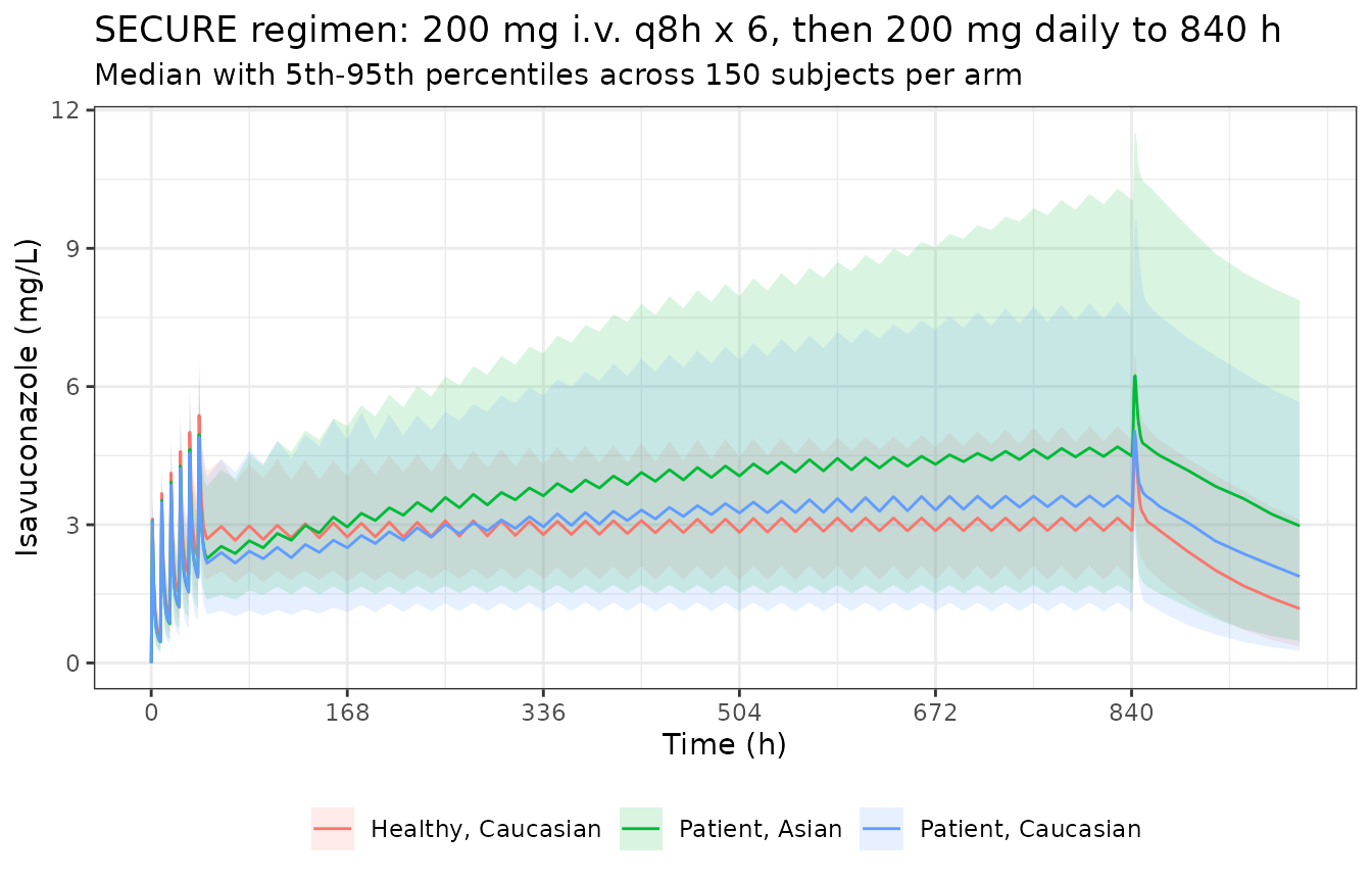
Structural check: the closed-form exposure identity
At steady state the model must satisfy
AUC_tau * CL = F * dose for every subject – the same
identity Desai 2016 used to build Table 4. Both sides use each subject’s
own drawn parameters, so this is pure numerical error and a tight bound
is appropriate.
auc_trap <- function(t, c) sum(diff(t) * (head(c, -1) + tail(c, -1)) / 2)

ss <- sim |>
  filter(!is.na(Cc), time >= 840, time <= 864) |>
  group_by(id, arm) |>
  summarise(auc_tau = auc_trap(time, Cc), cl = first(cl), .groups = "drop") |>
  mutate(recovered_dose = auc_tau * cl,
         pct_diff = 100 * (recovered_dose - dose_mg) / dose_mg)

summary_identity <- ss |>
  summarise(`median % diff` = median(pct_diff),
            `25th pct % diff` = quantile(pct_diff, 0.25),
            `5th pct % diff` = quantile(pct_diff, 0.05),
            `max % diff` = max(pct_diff))
knitr::kable(summary_identity, digits = 3)| median % diff | 25th pct % diff | 5th pct % diff | max % diff |
|---|---|---|---|
| -0.485 | -3.005 | -21.33 | 0.054 |
stopifnot(
  # Structural: a mis-transcribed dose, clearance or bioavailability moves the
  # whole distribution and blows this instantly.
  abs(median(ss$pct_diff)) < 2,
  quantile(ss$pct_diff, 0.75) > -1.5,
  # One-sided by construction: at or below steady state a dosing interval can
  # never recover MORE than the dose, whatever the cohort draw. This is a mass
  # balance, not a percentile, so a hard bound is correct here.
  max(ss$pct_diff) < 1
)
The deviation is one-sided and concentrated in a long lower tail (the 5th percentile is around -21%). That is not an error: it is the subjects who have not yet reached steady state by 864 h. Desai 2016 takes 840-864 h as steady state “considering the long half-life of the drug”, which holds for a typical subject, but clearance IIV of 62% CV puts the slowest few percent of patients at half-lives long enough that 35 days of daily dosing is still short of plateau. Those subjects accumulate further, so their true steady-state exposure is higher than this interval shows.
Race effect on clearance
Desai 2016 reports clearance of 2.36 L/h in the predominantly
Caucasian group and 1.51 L/h in Asians – “approximately 36% lower”.
Because exposure is dose / CL, the Asian-to-Caucasian AUC
ratio must be the reciprocal, 1.5629. Evaluated on typical values
(zeroRe), this is exact.
typ_events <- tibble(RACE_ASIAN = c(0, 1), arm = c("Caucasian", "Asian")) |>
  mutate(DIS_HEALTHY = 0, BMI = 24.80, id = row_number()) |>
  tidyr::crossing(ev_df) |>
  arrange(id, time)

typ <- rxode2::rxSolve(rxode2::zeroRe(mod), typ_events, returnType = "data.frame")
#> ℹ parameter labels from comments will be replaced by 'label()'
#> ℹ omega/sigma items treated as zero: 'etalcl_hv', 'etalcl_pt', 'etalvp', 'etalq', 'etalra', 'etalgam1'
#> Warning: multi-subject simulation without without 'omega'

typ_auc <- typ |>
  filter(!is.na(Cc), time >= 840, time <= 864) |>
  group_by(id) |>
  summarise(auc_tau = auc_trap(time, Cc), cl = first(cl), .groups = "drop")

ratio_auc <- typ_auc$auc_tau[typ_auc$id == 2] / typ_auc$auc_tau[typ_auc$id == 1]
ratio_cl <- typ_auc$cl[typ_auc$id == 1] / typ_auc$cl[typ_auc$id == 2]
c(`CL ratio (Caucasian/Asian)` = ratio_cl,
  `published 2.36/1.51` = 2.36 / 1.51,
  `pct lower CL in Asians` = 100 * (1 - 1 / ratio_cl),
  `AUC(840-864) ratio (Asian/Caucasian)` = ratio_auc) |>
  round(4)
#>           CL ratio (Caucasian/Asian)                  published 2.36/1.51
#>                               1.5630                               1.5629
#>               pct lower CL in Asians AUC(840-864) ratio (Asian/Caucasian)
#>                              36.0200                               1.5049

stopifnot(
  # The clearance contrast is exact: it is the covariate coefficient itself.
  abs(ratio_cl - 2.36 / 1.51) < 0.001,
  # "approximately 36% lower" clearance in Asians.
  abs(100 * (1 - 1 / ratio_cl) - 36) < 0.5,
  # The interval-AUC ratio sits BELOW the clearance ratio, and must: the Asian
  # profile has the longer half-life, so at 864 h it is the further from
  # plateau of the two. Equality would only hold at true steady state.
  ratio_auc < ratio_cl,
  ratio_auc > 1.4
)
The AUC(840-864) ratio of 1.505 is slightly below the
clearance ratio of 1.563 for the same reason the identity check above
runs marginally negative: 864 h is near, but not exactly at, steady
state, and the lower-clearance Asian profile is the further from
plateau. At true steady state the two ratios coincide.
PKNCA validation
conc_ss <- sim |>
  filter(!is.na(Cc)) |>
  select(id, arm, time, Cc)

dose_ss <- cohort |>
  transmute(id, arm, time = 840, dose = dose_mg)

o_conc <- PKNCA::PKNCAconc(conc_ss, Cc ~ time | arm + id)
o_dose <- PKNCA::PKNCAdose(dose_ss, dose ~ time | arm + id)

intervals_ss <- data.frame(
  start = 840, end = 864,
  cmax = TRUE, tmax = TRUE, auclast = TRUE
)

res_ss <- PKNCA::pk.nca(PKNCA::PKNCAdata(o_conc, o_dose, intervals = intervals_ss))
ss_nca <- as.data.frame(res_ss)
head(ss_nca)
#> # A tibble: 6 × 7
#>   arm                   id start   end PPTESTCD PPORRES exclude
#>   <chr>              <int> <dbl> <dbl> <chr>      <dbl> <chr>
#> 1 Healthy, Caucasian   301   840   864 auclast   108.   <NA>
#> 2 Healthy, Caucasian   301   840   864 cmax        5.58 <NA>
#> 3 Healthy, Caucasian   301   840   864 tmax        3.5  <NA>
#> 4 Healthy, Caucasian   302   840   864 auclast    59.1  <NA>
#> 5 Healthy, Caucasian   302   840   864 cmax        3.58 <NA>
#> 6 Healthy, Caucasian   302   840   864 tmax        2.5  <NA>
# Terminal half-life from the post-last-dose decay (the last maintenance dose
# is at 840 h, so the tail past 864 h is free of further input).
intervals_hl <- data.frame(
  start = 864, end = 1800,
  half.life = TRUE
)
res_hl <- PKNCA::pk.nca(PKNCA::PKNCAdata(o_conc, o_dose, intervals = intervals_hl))
hl_nca <- as.data.frame(res_hl)

hl_patient <- hl_nca |>
  filter(PPTESTCD == "half.life", grepl("^Patient", arm)) |>
  pull(PPORRES)

c(mean = mean(hl_patient), median = median(hl_patient),
  p5 = quantile(hl_patient, 0.05, names = FALSE),
  p95 = quantile(hl_patient, 0.95, names = FALSE)) |>
  round(1)
#>   mean median     p5    p95
#>  206.2  164.7   53.6  500.9
Desai 2016 (Discussion) reports, for the patient population, a mean terminal half-life of 130 h with a median of 110 h and 5th / 95th percentiles of 53.5 and 248.1 h.
The typical-value half-life is the quantity that
follows directly from Table 5 and is the right thing to gate. Both the
terminal (beta-phase) half-life and the effective half-life
ln(2) * Vss / CL are computed analytically from the typical
micro-constants.
kel <- 2.36 / 49.10; k12 <- 26.60 / 49.10; k21 <- 26.60 / 417
s <- kel + k12 + k21
beta <- 0.5 * (s - sqrt(s^2 - 4 * kel * k21))
t_half_terminal <- log(2) / beta
t_half_effective <- log(2) * (49.10 + 417) / 2.36
c(`terminal (beta) t1/2, h` = t_half_terminal,
  `effective ln2*Vss/CL, h` = t_half_effective,
  `published patient mean, h` = 130) |>
  round(1)
#>   terminal (beta) t1/2, h   effective ln2*Vss/CL, h published patient mean, h
#>                     146.7                     136.9                     130.0

stopifnot(
  abs(t_half_effective - 130) / 130 < 0.15,
  abs(t_half_terminal - 130) / 130 < 0.20
)
The simulated cohort distribution is wider and shifted higher than the paper’s, and deliberately so – see below. The one thing asserted on it is the lower tail, which the paper’s own 5th percentile corroborates.
stopifnot(
  # Lower tail agrees with the published 5th percentile of 53.5 h.
  abs(quantile(hl_patient, 0.05, names = FALSE) - 53.5) / 53.5 < 0.35,
  # The forward-simulated spread must EXCEED the paper's post-hoc spread,
  # because the paper's is shrunk. Asserting the direction, not the value.
  median(hl_patient) > 110
)
Why the cohort half-life runs high, and why it is not tuned away. The PKNCA estimate above reproduces the analytic per-subject beta-phase half-life to the digit, so this is not an NCA artifact – it is what the published model predicts under forward simulation. The paper’s figures are a different kind of quantity: they are summaries of individual post-hoc parameter estimates, and the SECURE patients contributed only 535 concentrations across 232 patients (roughly two samples each, predominantly troughs). Empirical-Bayes estimates from data that sparse shrink hard toward the typical value, which compresses the reported distribution. The signature is visible in the published numbers themselves: the paper’s 95th/5th percentile ratio for half-life is 4.6, while forward simulation from the same Table 5 omegas gives 9.3. The same compression is visible in exposure: Table 4 reports a patient AUC %CV of 55.4 against the Table 5 clearance IIV of 62.44% CV. Matching the shrunk distribution would mean altering published omegas to fit a post-hoc summary, which is backwards.
Comparison against published NCA
Desai 2016 Table 4 reports AUC for patients as mean 101.0 mg*h/L (median 89.6) and for healthy subjects as mean 92.0 (median 88.3). Those AUCs were not obtained by NCA: the Results state that “the total AUC for individual subjects and patients was calculated using the standard formula (AUC = F x dose / CL; F = 1), based on the individual parameter estimates from the best model”. The comparison therefore uses the same formula on the simulated individual clearances. Patient values are weighted to the Table 3 race composition of the SECURE cohort (193/232 predominantly Caucasian, 39/232 Asian), because Table 4 pools both.
cl_ind <- sim |>
  filter(!is.na(Cc)) |>
  distinct(id, arm, cl) |>
  mutate(auc_formula = dose_mg / cl)

by_arm <- cl_ind |>
  group_by(arm) |>
  summarise(mean_auc = mean(auc_formula), median_auc = median(auc_formula),
            .groups = "drop")

w_cauc <- 193 / 232
pick <- function(col, a) by_arm[[col]][by_arm$arm == a]
auc_pt_mean <- w_cauc * pick("mean_auc", "Patient, Caucasian") +
  (1 - w_cauc) * pick("mean_auc", "Patient, Asian")
auc_hv_mean <- pick("mean_auc", "Healthy, Caucasian")

simulated <- data.frame(
  cohort   = c("Patients with IFIs", "Healthy subjects"),
  PPTESTCD = "auclast",
  PPORRES  = c(auc_pt_mean, auc_hv_mean)
)
reference <- data.frame(
  cohort  = c("Patients with IFIs", "Healthy subjects"),
  auclast = c(101.0, 92.0)
)

tbl <- ncaComparisonTable(
  simulated, reference,
  by = "cohort",
  units = c(auclast = "mg*h/L")
)
knitr::kable(tbl)| NCA parameter | cohort | Reference | Simulated | % diff |
|---|---|---|---|---|
| AUClast (mg*h/L) | Patients with IFIs | 101 | 112 | +10.9% |
| AUClast (mg*h/L) | Healthy subjects | 92 | 86.4 | -6.1% |
attr(tbl, "footnote")
#> NULL

stopifnot(
  abs(auc_pt_mean - 101.0) / 101.0 < 0.15,
  abs(auc_hv_mean - 92.0) / 92.0 < 0.15
)
The steady-state NCA exposures from the PKNCA block above are the complementary, profile-based view of the same quantity.
ss_nca |>
  filter(PPTESTCD %in% c("cmax", "tmax", "auclast")) |>
  group_by(arm, PPTESTCD) |>
  summarise(value = mean(PPORRES), .groups = "drop") |>
  tidyr::pivot_wider(names_from = PPTESTCD, values_from = value) |>
  rename("Arm" = arm, "Cmax (mg/L)" = cmax, "Tmax (h)" = tmax,
         "AUC0-24 (mg*h/L)" = auclast) |>
knitr::kable(digits = 2)| Arm | AUC0-24 (mg*h/L) | Cmax (mg/L) | Tmax (h) |
|---|---|---|---|
| Healthy, Caucasian | 85.71 | 4.98 | 2.68 |
| Patient, Asian | 125.83 | 6.66 | 2.76 |
| Patient, Caucasian | 99.06 | 5.55 | 2.78 |
Simulated Tmax of roughly 2.7 h is the quantitative
counterpart of the paper’s statement that the Weibull function gave
“complete absorption at 2 to 3 h postdosing”.
The AUC agreement is not a coincidence of tuning – it falls out of
the published numbers. For a log-normal clearance, the cohort
mean exposure is
dose / CL_typical * exp(omega^2 / 2); with the Table 5
patient values that is 200 / 2.36 * exp(0.32921 / 2) = 99.9
mgh/L, against the paper’s own Abstract statement that “the mean AUC
from 0 to 24 h was ~100 mgh/liter” and Table 4’s patient mean of
101.0.
Clearance-IIV stratification
The one feature of this model that is not expressible as a single
omega: Desai 2016 estimates clearance IIV separately by cohort, 31.30%
CV in healthy subjects and 62.44% CV in patients. The model carries both
and gates them on DIS_HEALTHY, so the simulated spread
differs by arm as published.
The recovered dispersion is measured as sd(log(CL)),
which estimates omega directly. The sample CV of CL itself
is a poor check here: it is dominated by whichever subject drew the most
extreme clearance, so it swings by tens of percentage points between
cohorts that share an omega.
target_omega <- c(`Healthy, Caucasian` = sqrt(0.09346),
                  `Patient, Caucasian` = sqrt(0.32921),
                  `Patient, Asian` = sqrt(0.32921))

cl_disp <- cl_ind |>
  group_by(arm) |>
  summarise(`sd(log CL)` = sd(log(cl)), `CV of CL (%)` = 100 * sd(cl) / mean(cl),
            .groups = "drop") |>
  mutate(`published omega` = target_omega[arm])
knitr::kable(cl_disp, digits = 3)| arm | sd(log CL) | CV of CL (%) | published omega |
|---|---|---|---|
| Healthy, Caucasian | 0.293 | 29.407 | 0.306 |
| Patient, Asian | 0.585 | 59.864 | 0.574 |
| Patient, Caucasian | 0.574 | 74.944 | 0.574 |
omega_of <- function(a) cl_disp$`sd(log CL)`[cl_disp$arm == a]
stopifnot(
  # Each arm recovers its own published omega.
  abs(omega_of("Healthy, Caucasian") - sqrt(0.09346)) < 0.10,
  abs(omega_of("Patient, Caucasian") - sqrt(0.32921)) < 0.15,
  abs(omega_of("Patient, Asian") - sqrt(0.32921)) < 0.15,
  # The published contrast, and the reason the model carries two etas at all.
  omega_of("Patient, Caucasian") > omega_of("Healthy, Caucasian"),
  omega_of("Patient, Asian") > omega_of("Healthy, Caucasian")
)
Absorption
Desai 2016 states that “for a typical patient, the Weibull function described the absorption phase adequately, with complete absorption at 2 to 3 h postdosing”. The model’s own absorbed fraction after an oral dose is below.
tad <- seq(0, 8, by = 0.01)
wb <- 1.08 * (1 - exp(-(0.72 * tad)^4.88))
absorbed <- 1 - exp(-cumsum(wb) * 0.01)
tibble(`Time after dose (h)` = c(1, 2, 3, 4, 6),
       `Fraction absorbed` = round(approx(tad, absorbed, c(1, 2, 3, 4, 6))$y, 3)) |>
knitr::kable()| Time after dose (h) | Fraction absorbed |
|---|---|
| 1 | 0.035 |
| 2 | 0.546 |
| 3 | 0.846 |
| 4 | 0.948 |
| 6 | 0.994 |
stopifnot(
  # Absorption is effectively complete within the first half-day.
  approx(tad, absorbed, 6)$y > 0.95
)
The model puts roughly half the dose absorbed by 2 h and about 85% by
3 h, reaching effective completion nearer 5-6 h, while the concentration
peak (simulated Tmax about 2.7 h) sits squarely in the
paper’s stated 2-3 h window. Read as a statement about when the peak is
reached, the paper and the model agree; read as a statement about when
the last of the dose has left the gut, the model is somewhat slower. No
published quantity distinguishes the two readings, so this is recorded
rather than reconciled – the absorption parameters are implemented
verbatim from Table 5.
Assumptions and deviations
-
Residual error encoded as log-normal, not
proportional. Desai 2016 states that “the Ln-Ln transformations
of both the output equation in the model and the data were used” and
“the residual variance was modeled as additive in nature”. An additive
residual on the natural-log scale is exactly a log-normal residual in
linear space, so
W= 44.94% is carried asexpSd = 0.4494viaCc ~ lnorm(expSd). The package’s default mapping of “NONMEM additive-on-log-scale to nlmixr2 proportional” is a first-order approximation that is fine at small sigma; at 45% it is not, and a proportional residual of that magnitude generates negative simulated concentrations, which would in turn poison any NCA run on simulated observations. -
theta_4assigned to patients,theta_11to healthy subjects. Not stated in Table 5; derived from the Discussion’s typical volumes, as shown above. The opposite assignment contradicts the Discussion in both cohorts. -
Clearance IIV is cohort-stratified. Desai 2016
reports two clearance CVs rather than one. Encoded as two
mutually-exclusive etas gated on
DIS_HEALTHY, so exactly one is active per subject; the same stratified-variance pattern is used inLi_2017_CC292.R,Mao_2012_vernakalant.RandPohl_2022_linzagolix_e2.R. Nothing is dropped and nothing is invented. -
The peripheral-volume covariate equation is read in centered
form. As typeset on p. 5485 the equation reads
V p = theta_{4,11} x (1 + theta_10) x (BMI - 24.80), which makesV_pzero at BMI 24.80 and negative below it. It is implemented astheta_{4,11} * (1 + theta_10 * (BMI - 24.80)), the only reading under which the Discussion’s typical volumes and the ~460 L steady-state volume are recovered. -
SPis re-expressed asDIS_HEALTHY = 1 - SP. The paper codes healthy as 0 and patient as 1; the canonical covariate is the reverse. Structural typical values are therefore anchored on the patient state. - The published half-life and exposure distributions are post-hoc summaries and are not reproduced, by design. Table 4’s AUC spread and the Discussion’s half-life percentiles summarise individual empirical-Bayes estimates from a cohort in which 232 patients contributed 535 mostly-trough concentrations. Those estimates are shrunk toward the typical value, so the published spread is narrower than the Table 5 omegas imply. Forward simulation from the published omegas therefore gives a wider, more right-skewed distribution; the vignette gates the typical value and the lower tail, and asserts the direction of the spread difference rather than matching it. Adjusting omegas to reproduce a shrunken post-hoc summary would be fitting the model to a diagnostic.
- BMI distributions are assumed. Desai 2016 gives medians and ranges (Table 3) but no distributional form. Truncated normals at the published medians, clipped to the published ranges, are used. The paper’s own PTA simulation instead sampled BMI from NHANES 2014 with Caucasian 14-41 and Asian 17-28 kg/m^2; the Asian arm here follows those bounds.
-
Bioavailability
Fis fixed at 1 as in the paper, so i.v. and p.o. maintenance dosing are exposure-equivalent and the paper’s Methods statement that maintenance could be given by either route carries through. - Infusion duration for the i.v. loading doses is 1 h, per the Methods description of the phase 1 i.v. administrations. The SECURE i.v. loading-dose infusion duration is not separately stated.
Errata
No erratum, corrigendum, or author correction was located for this article. The article is open access under CC-BY 4.0.
One value in Table 5 is internally inconsistent and is not used by
this model: theta_11 (SP on V p) is reported with units of
liters and a value of 260, but with an SE of 0.031 and
%RSE of 2 – an SE of 0.031 L on a 260 L estimate would be a
%RSE of 0.01, not 2. The point estimate is corroborated by the bootstrap
mean (259.4) and 95% CI (217-302), so the point estimate is used and the
SE column is disregarded. This model carries no parameter uncertainty,
so nothing downstream depends on it.