Dorzagliatin (Wang 2023)

Model and source

• Citation: Wang K, Feng L, Zhang J, Zou Q, Xu F, Sun Z, Tang F, Chen L. (2023). Population pharmacokinetic analysis of dorzagliatin in healthy subjects and patients with type 2 diabetes mellitus. Clin Pharmacokinet 62(10):1419-1430. doi:10.1007/s40262-023-01286-8
• Article: https://doi.org/10.1007/s40262-023-01286-8
• Supplement (Tables S1-S4): https://static-content.springer.com/esm/art%3A10.1007%2Fs40262-023-01286-8/MediaObjects/40262_2023_1286_MOESM1_ESM.docx

Dorzagliatin (HMS5552) is a first-in-class dual-acting glucokinase activator approved in China in September 2022 for adults with type 2 diabetes mellitus (T2DM), as monotherapy and as an add-on to metformin. Wang 2023 pooled six trials from the Hua Medicine development programme into a single population PK analysis to quantify the influence of demographic, hepatic and renal covariates on dorzagliatin exposure.

The structural model is a two-compartment model with sequential zero-order then first-order oral absorption and first-order elimination: the dose enters the depot at a constant rate over a window of duration D1, and the depot then drains into the central compartment first-order at ka. All disposition parameters are apparent (CL/F, Vc/F, Q/F, Vp/F) because only oral data were analysed; bioavailability was not estimated and is implicitly 1.

mod <- readModelDb("Wang_2023_dorzagliatin")
mod
#> function() {
#>   description <- paste(
#>     "Two-compartment population PK model for oral dorzagliatin (HMS5552,",
#>     "a first-in-class dual-acting glucokinase activator approved in China",
#>     "for type 2 diabetes mellitus) in healthy subjects and patients with",
#>     "T2DM (Wang 2023; N = 1062 subjects, 7686 concentrations pooled from",
#>     "six clinical trials). Disposition is a two-compartment model with",
#>     "sequential zero-order then first-order oral absorption (dose enters",
#>     "the depot over a zero-order window of duration D1 = 0.418 h, then is",
#>     "absorbed first-order at ka = 3.29 h^-1) and first-order elimination",
#>     "from the central compartment. Typical values for a 69 kg, 55-year-old",
#>     "male with AST 18 U/L enrolled in the later-phase studies are CL/F =",
#>     "10.4 L/h, Vc/F = 80.6 L, Q/F = 3.02 L/h and Vp/F = 26.5 L. CL/F",
#>     "carries three power covariate effects plus one study indicator:",
#>     "(WT/69)^0.255, (AST/18)^-0.103, (AGE/55)^-0.135 and a multiplicative",
#>     "exp(0.203) = 1.23 uplift for the three early-phase studies",
#>     "(HMM0102 / HMM0103 / HMM0110), which the paper attributes to a",
#>     "formulation / bioavailability difference that could not be resolved",
#>     "as an F effect. Vc/F carries (WT/69)^0.553 and a multiplicative",
#>     "exp(-0.170) = 0.843 factor in females (15.7% lower than males). D1",
#>     "carries exp(0.816) = 2.26 when food is consumed at least 1 h after",
#>     "dosing rather than 0.5 h after dosing. Because sex acts only on Vc/F",
#>     "and the meal-timing effect only on D1, neither changes steady-state",
#>     "AUCtau (the paper reports 0.01% and 0% respectively) while both shift",
#>     "Cmax,ss and Cmin,ss. Inter-individual variability is a correlated",
#>     "CL/F-Vc/F block (approximate CV 22.5% and 14.9%; covariance 0.0181)",
#>     "plus independent terms on Vp/F (48.8%) and D1 (82.8%); ka and Q/F",
#>     "carry no IIV. Residual error is combined additive plus proportional",
#>     "(109 ng/mL and 32.9%).",
#>     sep = " "
#>   )
#>   reference <- paste(
#>     "Wang K, Feng L, Zhang J, Zou Q, Xu F, Sun Z, Tang F, Chen L. (2023).",
#>     "Population pharmacokinetic analysis of dorzagliatin in healthy",
#>     "subjects and patients with type 2 diabetes mellitus.",
#>     "Clin Pharmacokinet 62(10):1419-1430.",
#>     "doi:10.1007/s40262-023-01286-8",
#>     sep = " "
#>   )
#>   vignette <- "Wang_2023_dorzagliatin"
#>   units    <- list(time = "h", dosing = "mg", concentration = "ng/mL")
#> 
#>   # Issue #482: what each ODE state holds, in what amount units, in what
#>   # biological matrix. Derived mechanically; verified = FALSE means it has
#>   # NOT been checked against the source paper.
#>   compartmentData <- list(
#>     depot       = list(analyte = "dorzagliatin", units = "mg", specimen = "administration site", verified = FALSE),
#>     central     = list(analyte = "dorzagliatin", units = "mg", specimen = "plasma", verified = FALSE),
#>     peripheral1 = list(analyte = "dorzagliatin", units = "mg", specimen = "plasma", verified = FALSE)
#>   )
#> 
#>   covariateData <- list(
#>     WT = list(
#>       description        = "Total body weight",
#>       units              = "kg",
#>       type               = "continuous",
#>       reference_category = NULL,
#>       notes              = paste(
#>         "Baseline, time-fixed. Overall population median 69.0 kg",
#>         "(range 40.0-110; Wang 2023 Table 2 'TBW, kg' Overall column),",
#>         "which is the normalization constant used by both covariate",
#>         "relationships. Retained on CL/F and Vc/F in the final model as",
#>         "power effects (WT/69)^0.255 and (WT/69)^0.553 -- the paper prints",
#>         "these in the algebraically identical exp(theta * log(WT/69))",
#>         "form (Wang 2023 Table 3 footnote equations). Note that neither",
#>         "exponent is the allometric 0.75 / 1.0 pair; both were estimated",
#>         "(RSE 19.4% and 9.94%). Wang 2023 Discussion reports the",
#>         "resulting 10th-90th percentile spread (55 kg and 83 kg) as",
#>         "-5.63% to +4.83% on CL/F and -11.8% to +10.8% on Vc/F."
#>       ),
#>       source_name        = "TBW"
#>     ),
#>     AGE = list(
#>       description        = "Age at baseline",
#>       units              = "years",
#>       type               = "continuous",
#>       reference_category = NULL,
#>       notes              = paste(
#>         "Baseline, time-fixed. Overall population median 55.0 years",
#>         "(range 19.0-74.2; Wang 2023 Table 2 'AGE, year' Overall column),",
#>         "used as the normalization constant. Retained on CL/F as the",
#>         "power effect (AGE/55)^-0.135, i.e. older subjects have lower",
#>         "CL/F and therefore higher exposure. Wang 2023 Discussion",
#>         "reports +4.06% (41 years) to -2.44% (66 years) on CL/F across",
#>         "the 10th-90th percentiles. No subject was younger than 19 or",
#>         "older than 74.2 years, so the relationship is not established",
#>         "in pediatric or very elderly subjects."
#>       ),
#>       source_name        = "AGE"
#>     ),
#>     AST = list(
#>       description        = "Baseline aspartate aminotransferase",
#>       units              = "U/L",
#>       type               = "continuous",
#>       reference_category = NULL,
#>       notes              = paste(
#>         "Baseline, time-fixed. Overall population median 18.0 U/L",
#>         "(range 8.00-74.0; Wang 2023 Table 2 'AST, U/L' Overall column),",
#>         "used as the normalization constant. Reported by the paper in",
#>         "U/L, matching the canonical SI unit (the source uses U/L and",
#>         "IU/L interchangeably; the supplement quotes the AST upper limit",
#>         "of normal as 40 IU/L). Retained on CL/F as the power effect",
#>         "(AST/18)^-0.103: higher AST (poorer hepatocellular integrity)",
#>         "gives lower CL/F and higher exposure. Wang 2023 Discussion",
#>         "reports +3.41% (13 U/L) to -4.45% (28 U/L) on CL/F across the",
#>         "10th-90th percentiles. AST is the only retained hepatic marker;",
#>         "ALT and total bilirubin were screened and dropped."
#>       ),
#>       source_name        = "AST"
#>     ),
#>     SEXF = list(
#>       description        = "Female sex indicator",
#>       units              = "(binary)",
#>       type               = "binary",
#>       reference_category = "0 (male)",
#>       notes              = paste(
#>         "Time-fixed per subject. The source column GEND is coded 1 =",
#>         "female, 0 = male (Wang 2023 Table 3 footnote: 'GEND: 1 for",
#>         "female, 0 for male'), which is exactly the canonical SEXF",
#>         "orientation -- no value transformation is required. Cohort",
#>         "397 / 1062 female (37.4%) per Wang 2023 Table 2. Retained on",
#>         "Vc/F only as a multiplicative exp(-0.170) = 0.843 factor,",
#>         "i.e. females have 15.7% lower Vc/F than males (Wang 2023",
#>         "Discussion). Because sex does not act on CL/F, steady-state",
#>         "AUCtau is essentially unchanged between sexes (0.01% per",
#>         "Wang 2023 Section 3.3) while Cmax,ss is 9.09% higher and",
#>         "Cmin,ss 11.6% lower in females."
#>       ),
#>       source_name        = "GEND"
#>     ),
#>     STUDY_DORZA_EARLY = list(
#>       description        = "Early-phase dorzagliatin study indicator (HMM0102 / HMM0103 / HMM0110)",
#>       units              = "(binary)",
#>       type               = "binary",
#>       reference_category = "0 (later-phase studies HMM0201 / HMM0301 / HMM0302)",
#>       notes              = paste(
#>         "Time-fixed per subject; set from the trial identifier. 1 = the",
#>         "subject was enrolled in study HMM0102 (NCT02077452), HMM0103",
#>         "(NCT02386982) or HMM0110 (NCT04324424); 0 = HMM0201",
#>         "(NCT02561338), HMM0301 (NCT03173391) or HMM0302 (NCT03141073).",
#>         "Wang 2023 Table 3 footnote: 'Study: 1 for study 102/103/110, 0",
#>         "for others'. Enters CL/F as exp(0.203 * STUDY_DORZA_EARLY) =",
#>         "a 1.23-fold (22.5% higher) apparent clearance in the",
#>         "early-phase studies. Wang 2023 Discussion paragraph 2 explains",
#>         "the mechanism: those studies showed systematically lower",
#>         "exposure, plausibly a formulation difference (studies 301 and",
#>         "302 used near-commercial preparations), but 'the model was",
#>         "unable to correct for prediction bias by bioavailability' in",
#>         "the sparsely-sampled later studies, so the between-trial",
#>         "difference was absorbed into CL/F instead of F."
#>       ),
#>       source_name        = "Study"
#>     ),
#>     MEAL_DELAY_1H = list(
#>       description        = "Delayed-meal indicator: food consumed at least 1 h after dosing rather than 0.5 h after dosing",
#>       units              = "(binary)",
#>       type               = "binary",
#>       reference_category = "0 (food consumed 0.5 h after dosing)",
#>       notes              = paste(
#>         "Per-dose-record indicator. 1 = the subject started eating at",
#>         "least 1 h after taking the dose; 0 = the subject started eating",
#>         "0.5 h after taking the dose (Wang 2023 Table 3 footnote:",
#>         "'FOOD: 0 and 1 for the time of food consumption after 0.5 h and",
#>         ">= 1 h of drug administration, respectively'). Both levels are",
#>         "fed states -- this covariate encodes the dose-to-meal interval,",
#>         "not the presence or the fat content of a meal, so it is distinct",
#>         "from FED, FED_HIGHFAT and FED_LOWFAT. Retained on D1 only, as",
#>         "the multiplicative factor exp(0.816) = 2.26: waiting at least",
#>         "1 h before eating more than doubles the zero-order absorption",
#>         "window (0.418 h -> 0.945 h). Because D1 does not affect CL/F,",
#>         "steady-state AUCtau is unchanged and Cmax,ss / Cmin,ss shift by",
#>         "only -1.26% / +2.71% (Wang 2023 Section 3.3). Note that Wang",
#>         "2023 Table 3 mislabels this row as 'D1,FOOD -- Influence of",
#>         "food consumption time on CL/F'; the printed equation and the",
#>         "parameter name both place the effect on D1, and the Discussion",
#>         "confirms 'patients with time to food consumption of >= 1 h",
#>         "after drug administration had higher D1'."
#>       ),
#>       source_name        = "FOOD"
#>     )
#>   )
#> 
#>   covariatesDataExcluded <- list(
#>     BMI = list(
#>       description        = "Baseline body mass index",
#>       units              = "kg/m^2",
#>       type               = "continuous",
#>       reference_category = NULL,
#>       notes              = paste(
#>         "Screened in the stepwise forward-inclusion / backward-",
#>         "elimination covariate search (Wang 2023 Section 2.4) but not",
#>         "retained in the final model. Overall median 25.2 kg/m^2",
#>         "(range 18.2-34.9) per Table 2. Wang 2023 Section 3.4 and",
#>         "Table S1 report the geometric-mean exposure difference across",
#>         "BMI quartiles as only -10% to +5.57% relative to the overall",
#>         "population, driven by correlated covariates rather than a",
#>         "retained BMI effect."
#>       ),
#>       source_name        = "BMI"
#>     ),
#>     BSA = list(
#>       description        = "Baseline body surface area",
#>       units              = "m^2",
#>       type               = "continuous",
#>       reference_category = NULL,
#>       notes              = paste(
#>         "Screened (Wang 2023 Section 2.4 covariate list) but not",
#>         "retained; body weight was the size descriptor kept on both",
#>         "CL/F and Vc/F. Not tabulated in Wang 2023 Table 2."
#>       ),
#>       source_name        = "BSA"
#>     ),
#>     ALB = list(
#>       description        = "Baseline serum albumin",
#>       units              = "g/L",
#>       type               = "continuous",
#>       reference_category = NULL,
#>       notes              = paste(
#>         "Screened but not retained. Overall median 46.2 g/L (range",
#>         "33.2-57.0) per Wang 2023 Table 2; already in canonical SI",
#>         "units, so no conversion is needed."
#>       ),
#>       source_name        = "ALB"
#>     ),
#>     ALT = list(
#>       description        = "Baseline alanine aminotransferase",
#>       units              = "U/L",
#>       type               = "continuous",
#>       reference_category = NULL,
#>       notes              = paste(
#>         "Screened but not retained; AST was the hepatic marker kept on",
#>         "CL/F. Overall median 19.0 U/L (range 2.50-110) per Wang 2023",
#>         "Table 2. Wang 2023 Section 3.2 states explicitly that ALT",
#>         "'had no significant effect on the pharmacokinetics of",
#>         "dorzagliatin'."
#>       ),
#>       source_name        = "ALT"
#>     ),
#>     CREAT = list(
#>       description        = "Baseline serum creatinine",
#>       units              = "umol/L",
#>       type               = "continuous",
#>       reference_category = NULL,
#>       notes              = paste(
#>         "Screened but not retained. Overall median 67.0 umol/L (range",
#>         "35.0-943) per Wang 2023 Table 2; the extreme upper end comes",
#>         "from study HMM0110, the dedicated renal-impairment study",
#>         "(median 235 umol/L in that cohort). Already in canonical SI",
#>         "units."
#>       ),
#>       source_name        = "CR"
#>     ),
#>     CRCL = list(
#>       description        = "Baseline creatinine clearance",
#>       units              = "mL/min",
#>       type               = "continuous",
#>       reference_category = NULL,
#>       notes              = paste(
#>         "Screened but not retained. Not tabulated in Wang 2023 Table 2",
#>         "(the reported renal marker is serum creatinine). Wang 2023",
#>         "Section 3.2 states creatinine clearance 'had no significant",
#>         "effect'; the Discussion adds that a two-part renal-impairment",
#>         "study found only limited exposure differences between ESRD",
#>         "subjects and healthy volunteers (geometric mean ratio 0.81 for",
#>         "Cmax and 1.11 for AUC), so no dose adjustment is needed at any",
#>         "stage of renal impairment. The paper does not state whether",
#>         "the screened column was BSA-normalized."
#>       ),
#>       source_name        = "CRCL"
#>     ),
#>     TBILI = list(
#>       description        = "Baseline total bilirubin",
#>       units              = "umol/L",
#>       type               = "continuous",
#>       reference_category = NULL,
#>       notes              = paste(
#>         "Screened but not retained. Overall median 10.0 umol/L (range",
#>         "1.25-40.0) per Wang 2023 Table 2; already in canonical SI",
#>         "units. Used together with AST to assign the FDA hepatic-",
#>         "function categories in Wang 2023 Table S3 (the supplement",
#>         "quotes upper limits of normal of 20.5 umol/L for total",
#>         "bilirubin and 40 IU/L for AST), but it carries no retained",
#>         "effect on any PK parameter."
#>       ),
#>       source_name        = "TBIL"
#>     )
#>   )
#> 
#>   population <- list(
#>     species         = "human",
#>     n_subjects      = 1062L,
#>     n_studies       = 6L,
#>     n_observations  = 7686L,
#>     age_range       = "19.0-74.2 years",
#>     age_median      = "55.0 years",
#>     weight_range    = "40.0-110 kg",
#>     weight_median   = "69.0 kg",
#>     bmi_median      = "25.2 kg/m^2 (range 18.2-34.9)",
#>     sex_female_pct  = 37.4,
#>     race_ethnicity  = c(Asian = 100),
#>     disease_state   = paste(
#>       "Pooled cohort of healthy volunteers and adult patients with type 2",
#>       "diabetes mellitus from six trials (Wang 2023 Table 1): two phase I",
#>       "studies (HMM0102 / NCT02077452 multiple ascending dose;",
#>       "HMM0103 / NCT02386982 28-day beta-cell-function study), one phase",
#>       "II dose-ranging study (HMM0201 / NCT02561338), two phase III",
#>       "studies (HMM0301 / NCT03173391 monotherapy in drug-naive patients;",
#>       "HMM0302 / NCT03141073 add-on to metformin), and one open-label",
#>       "renal-impairment study with matched healthy volunteers",
#>       "(HMM0110 / NCT04324424)."
#>     ),
#>     dose_range      = paste(
#>       "25-400 mg/day orally: 25, 50, 100, 150 and 200 mg twice daily",
#>       "(HMM0102); 75 mg once or twice daily and 100 mg once daily",
#>       "(HMM0103, HMM0201, HMM0301, HMM0302); 25 mg twice daily",
#>       "(HMM0110). The approved and pivotal-trial regimen is 75 mg",
#>       "twice daily."
#>     ),
#>     regions         = "China (all six trials were conducted by Hua Medicine in Chinese subjects)",
#>     hepatic_function = paste(
#>       "Per the FDA hepatic-impairment categories derived from AST and",
#>       "total bilirubin (Wang 2023 Table S3): normal 974 / 92.2%, mild",
#>       "77 / 7.29%, moderate 5 / 0.473%, severe 0. Baseline AST median",
#>       "18.0 U/L (8.00-74.0), ALT 19.0 U/L (2.50-110), albumin 46.2 g/L",
#>       "(33.2-57.0), total bilirubin 10.0 umol/L (1.25-40.0)."
#>     ),
#>     renal_function  = paste(
#>       "Baseline serum creatinine median 67.0 umol/L (35.0-943); the wide",
#>       "upper range comes from the dedicated renal-impairment study",
#>       "HMM0110 (cohort median 235 umol/L), which enrolled subjects",
#>       "through end-stage renal disease. Wang 2023 Table S4 groups the",
#>       "analysis population as normal 936 and mild 109 by eGFR."
#>     ),
#>     notes           = paste(
#>       "Wang 2023 Table 2 summarises baseline demographics by study and",
#>       "overall; Table 1 lists the study designs, dose regimens and PK",
#>       "sampling schedules. Parameter estimates implemented here are the",
#>       "final-model 'Estimate (%RSE)' column of Wang 2023 Table 3, fit in",
#>       "NONMEM 7.4.3 with FOCE-with-interaction and confirmed by a",
#>       "1000-replicate nonparametric bootstrap whose medians agree with",
#>       "the point estimates to within rounding. Race is not tabulated;",
#>       "all six trials were conducted in China, so the cohort is recorded",
#>       "here as Asian."
#>     )
#>   )
#> 
#>   ini({
#>     # -----------------------------------------------------------------------
#>     # Structural PK -- Wang 2023 Table 3, 'Final model Estimate (%RSE)'
#>     # column. All disposition parameters are apparent (i.e. /F): the paper
#>     # analysed oral data only and did not estimate an absolute
#>     # bioavailability, so F is implicitly 1 and no lfdepot term is used.
#>     # Typical values correspond to a 69 kg, 55-year-old male with AST
#>     # 18 U/L enrolled in the later-phase studies (Wang 2023 Section 3.2).
#>     # Units are hour / L / L/h; concentration is converted to ng/mL inside
#>     # model() (see the observation comment there).
#>     # -----------------------------------------------------------------------
#>     lcl <- log(10.4)  ; label("Apparent total clearance CL/F (L/h)")                        # Wang 2023 Table 3 CL/F = 10.4 L/h (RSE 0.923%, 95% CI 10.2-10.6; bootstrap median 10.4)
#>     lvc <- log(80.6)  ; label("Apparent central volume of distribution Vc/F (L)")           # Wang 2023 Table 3 Vc/F = 80.6 L (RSE 1.23%, 95% CI 78.7-82.6; bootstrap median 80.6)
#>     lq  <- log(3.02)  ; label("Apparent inter-compartmental clearance Q/F (L/h)")           # Wang 2023 Table 3 Q/F = 3.02 L/h (RSE 9.70%, 95% CI 2.50-3.66; bootstrap median 3.01)
#>     lvp <- log(26.5)  ; label("Apparent peripheral volume of distribution Vp/F (L)")        # Wang 2023 Table 3 Vp/F = 26.5 L (RSE 6.95%, 95% CI 23.1-30.4; bootstrap median 26.7)
#>     lka <- log(3.29)  ; label("First-order absorption rate constant ka (1/h)")              # Wang 2023 Table 3 Ka = 3.29 1/h (RSE 5.30%, 95% CI 2.96-3.65; bootstrap median 3.29)
#>     ld1 <- log(0.418) ; label("Zero-order absorption input duration D1 (h)")                # Wang 2023 Table 3 D1 = 0.418 h (RSE 7.49%, 95% CI 0.361-0.484; bootstrap median 0.415)
#> 
#>     # -----------------------------------------------------------------------
#>     # Covariate effects. Wang 2023 prints the three final-model covariate
#>     # relations immediately below Table 3 as:
#>     #
#>     #   CL/F = 10.4 * exp(0.203 * Study + 0.255 * log(BW/69)
#>     #                     - 0.103 * log(AST/18) - 0.135 * log(AGE/55) + eta_CL)
#>     #   Vc/F = 80.6 * exp(0.553 * log(BW/69) - 0.170 * GEND + eta_Vc)
#>     #   D1   = 0.418 * exp(0.816 * FOOD + eta_D1)
#>     #
#>     # The continuous terms exp(theta * log(cov/ref)) are written below in the
#>     # algebraically identical power form (cov/ref)^theta, which is the
#>     # nlmixr2lib convention. The binary terms stay in exp() form.
#>     #
#>     # Table 3 reports the three binary/indicator effects already
#>     # exponentiated, which is how the two representations reconcile:
#>     #   CL_STUDY  = 1.23  = exp(0.203)   -> +22.5% CL/F in the early studies
#>     #   Vc,GEND   = 0.843 = exp(-0.170)  -> -15.7% Vc/F in females
#>     #   D1,FOOD   = 2.26  = exp(0.816)   -> +126% D1 when eating >= 1 h post-dose
#>     # while the continuous power exponents are tabulated on the log scale
#>     # directly (CL_BW 0.255, Vc,BW 0.553, CL_AST -0.103, CL_AGE -0.135).
#>     # Every one of these coefficients was checked by reproducing the paper's
#>     # own reported percentage changes -- see the vignette source-trace table.
#>     # -----------------------------------------------------------------------
#>     e_study_dorza_early_cl <- 0.203  ; label("Early-phase-study effect on CL/F (log-scale indicator coefficient)")           # Wang 2023 Table 3 footnote equation '0.203 x Study'; Table 3 CL_STUDY = 1.23 = exp(0.203) (RSE 2.39%, 95% CI 1.17-1.28)
#>     e_wt_cl                <- 0.255  ; label("Power effect of body weight on CL/F (unitless, reference 69 kg)")             # Wang 2023 Table 3 CL_BW = 0.255 (RSE 19.4%, 95% CI 0.158-0.352); footnote equation '0.255 x log(BW/69)'
#>     e_ast_cl               <- -0.103 ; label("Power effect of AST on CL/F (unitless, reference 18 U/L)")                    # Wang 2023 Table 3 CL_AST = -0.103 (RSE 21.3%, 95% CI -0.146 to -0.0601); footnote equation '-0.103 x log(AST/18)'
#>     e_age_cl               <- -0.135 ; label("Power effect of age on CL/F (unitless, reference 55 years)")                  # Wang 2023 Table 3 CL_AGE = -0.135 (RSE 28.5%, 95% CI -0.211 to -0.0599); footnote equation '-0.135 x log(AGE/55)'
#>     e_wt_vc                <- 0.553  ; label("Power effect of body weight on Vc/F (unitless, reference 69 kg)")             # Wang 2023 Table 3 Vc,BW = 0.553 (RSE 9.94%, 95% CI 0.445-0.661); footnote equation '0.553 x log(BW/69)'
#>     # NOTE on e_sexf_vc: the paper quotes this effect three ways that do not
#>     # round to one another -- equation coefficient -0.170, Table 3
#>     # Vc,GEND = 0.843, and Discussion "females were 15.7% lower". But
#>     # exp(-0.170) = 0.84366 (rounds to 0.844, not 0.843) and
#>     # log(0.843) = -0.170788. Both are roundings of the same underlying
#>     # estimate (~-0.1708) at different precisions. The equation coefficient is
#>     # used here per the printed-equation-governs convention; the resulting
#>     # female/male Vc/F ratio is 0.8437 (-15.63%) rather than the quoted -15.7%.
#>     # See the vignette Errata for the measured consequence on Cmax,ss/Cmin,ss
#>     # (all differences < 0.07 percentage points).
#>     e_sexf_vc              <- -0.170 ; label("Female-sex effect on Vc/F (log-scale indicator coefficient)")                 # Wang 2023 Table 3 footnote equation '-0.170 x GEND'; cf. Table 3 Vc,GEND = 0.843 (RSE 1.74%, 95% CI 0.815-0.873)
#>     e_meal_delay_1h_d1     <- 0.816  ; label("Delayed-meal effect on D1 (log-scale indicator coefficient)")                 # Wang 2023 Table 3 footnote equation '0.816 x FOOD'; Table 3 D1,FOOD = 2.26 = exp(0.816) (RSE 12.8%, 95% CI 1.76-2.91)
#> 
#>     # -----------------------------------------------------------------------
#>     # Inter-individual variability. Wang 2023 Table 3 reports IIV_CL 22.5%,
#>     # IIV_Vc 14.9%, IIV_Vp 48.8% and IIV_D1 82.8% with the footnote "IIV for
#>     # CL, Vc, Vp, D1, and proportional error are reported as approximate
#>     # CV%". "Approximate" identifies the sqrt-of-variance convention
#>     # CV% = 100 * sqrt(omega^2), i.e. omega = CV/100, rather than the exact
#>     # log-normal CV% = 100 * sqrt(exp(omega^2) - 1); the exact form would not
#>     # be described as an approximation. The two readings differ negligibly
#>     # here in any case (omega_CL 0.2250 vs 0.2222).
#>     #
#>     # Variances entered below are therefore (CV/100)^2:
#>     #   var(CL) = 0.225^2 = 0.050625      var(Vc) = 0.149^2 = 0.022201
#>     #   var(Vp) = 0.488^2 = 0.238144      var(D1) = 0.828^2 = 0.685584
#>     # The CL-Vc covariance is taken directly from Table 3 Cor_CL,Vc =
#>     # 0.0181, which is labelled "Covariance (CL, Vc)" and is already on the
#>     # omega scale. It implies a correlation of
#>     # 0.0181 / (0.225 * 0.149) = 0.540, and satisfies the positive-definite
#>     # bound |cov| < sqrt(var_CL * var_Vc) = 0.0335.
#>     #
#>     # ka and Q/F have no IIV term in Wang 2023 Table 3 and none is invented
#>     # here (the model is encoded exactly as published).
#>     # -----------------------------------------------------------------------
#>     etalcl + etalvc ~ c(0.050625,
#>                         0.0181, 0.022201)                                                                                   # Wang 2023 Table 3: IIV_CL 22.5% CV -> var 0.050625; Cor_CL,Vc = 0.0181 (RSE 10.9%); IIV_Vc 14.9% CV -> var 0.022201
#>     etalvp ~ 0.238144                                                                                                       # Wang 2023 Table 3 IIV_Vp = 48.8% CV (RSE 9.25%, 95% CI 38.9-57.0) -> var 0.488^2
#>     etald1 ~ 0.685584                                                                                                       # Wang 2023 Table 3 IIV_D1 = 82.8% CV (RSE 8.16%, 95% CI 68.3-95.2) -> var 0.828^2
#> 
#>     # -----------------------------------------------------------------------
#>     # Residual error: combined additive plus proportional (Wang 2023 Section
#>     # 2.3, "The final residual error model included additive and
#>     # proportional error terms"). Both Table 3 rows are reported on the SD
#>     # scale in their own units -- 'sigma1 (%) Proportional error 32.9' and
#>     # 'sigma2 (ng/mL) Additive error 109' -- so they are used directly as
#>     # propSd and addSd rather than being square-rooted.
#>     # -----------------------------------------------------------------------
#>     propSd <- 0.329 ; label("Proportional residual error (fraction)")     # Wang 2023 Table 3 sigma1 = 32.9% (RSE 1.34%, 95% CI 32.0-33.7; bootstrap median 32.8)
#>     addSd  <- 109   ; label("Additive residual error (ng/mL)")            # Wang 2023 Table 3 sigma2 = 109 ng/mL (RSE 1.38%, 95% CI 106-112; bootstrap median 109)
#>   })
#> 
#>   model({
#>     # ---------------------------------------------------------------------
#>     # 1. Individual PK parameters.
#>     #
#>     # CL/F carries the early-study indicator plus three power covariate
#>     # effects; Vc/F carries body weight and female sex; Vp/F, Q/F and ka
#>     # are covariate-free. D1 carries the meal-timing indicator.
#>     #
#>     # Reference (normalization) values are the overall population medians
#>     # from Wang 2023 Table 2: 69 kg, 18 U/L AST, 55 years. At the reference
#>     # covariate vector with STUDY_DORZA_EARLY = 0, SEXF = 0 and
#>     # MEAL_DELAY_1H = 0 every multiplier collapses to 1 and the parameters
#>     # reduce to the Table 3 typical values.
#>     # ---------------------------------------------------------------------
#>     cl <- exp(lcl + etalcl) *
#>       exp(e_study_dorza_early_cl * STUDY_DORZA_EARLY) *
#>       (WT / 69)^e_wt_cl *
#>       (AST / 18)^e_ast_cl *
#>       (AGE / 55)^e_age_cl
#>     vc <- exp(lvc + etalvc) *
#>       exp(e_sexf_vc * SEXF) *
#>       (WT / 69)^e_wt_vc
#>     vp <- exp(lvp + etalvp)
#>     q  <- exp(lq)
#>     ka <- exp(lka)
#>     d1 <- exp(ld1 + etald1) * exp(e_meal_delay_1h_d1 * MEAL_DELAY_1H)
#> 
#>     # 2. Micro-constants for the two-compartment system.
#>     kel <- cl / vc
#>     k12 <- q  / vc
#>     k21 <- q  / vp
#> 
#>     # ---------------------------------------------------------------------
#>     # 3. Two-compartment ODE system with sequential zero-order then
#>     #    first-order absorption (Wang 2023 Section 2.3 / 3.2). The dose is
#>     #    delivered into `depot` at a constant rate over the zero-order
#>     #    window of duration D1, and `depot` then drains into `central`
#>     #    first-order at ka. Dose records must therefore carry rate = -2 so
#>     #    that rxode2 uses the model's dur(depot); a plain bolus would
#>     #    collapse the zero-order phase and bias Cmax.
#>     # ---------------------------------------------------------------------
#>     d/dt(depot)       <- -ka * depot
#>     d/dt(central)     <-  ka * depot - kel * central - k12 * central + k21 * peripheral1
#>     d/dt(peripheral1) <-  k12 * central - k21 * peripheral1
#> 
#>     dur(depot) <- d1
#> 
#>     # ---------------------------------------------------------------------
#>     # 4. Observation. Dose is in mg and vc in L, so central / vc is mg/L
#>     #    (= ug/mL); multiplying by 1000 gives ng/mL, the assay unit used
#>     #    throughout Wang 2023 (Table 3 additive residual error 109 ng/mL;
#>     #    Table S1-S4 steady-state exposures ~1088 ng/mL Cmax,ss and
#>     #    ~7153 ng*h/mL AUCtau,ss at 75 mg twice daily).
#>     # ---------------------------------------------------------------------
#>     Cc <- central / vc * 1000
#>     Cc ~ add(addSd) + prop(propSd)
#>   })
#> }
#> <environment: 0x559a3eaad948>

Population

The analysis dataset comprised 7686 plasma concentrations from 1062 subjects across six trials (Wang 2023 Table 1): two phase I studies (HMM0102 / NCT02077452 multiple ascending dose; HMM0103 / NCT02386982 28-day beta-cell-function study), one phase II dose-ranging study (HMM0201 / NCT02561338), two phase III studies (HMM0301 / NCT03173391 monotherapy in drug-naive patients; HMM0302 / NCT03141073 add-on to metformin), and one open-label renal-impairment study with matched healthy volunteers (HMM0110 / NCT04324424). Doses ranged from 25 to 400 mg/day; the approved and pivotal-trial regimen is 75 mg twice daily.

Baseline demographics (Wang 2023 Table 2, Overall column, median with min-max): age 55.0 years (19.0-74.2), total body weight 69.0 kg (40.0-110), BMI 25.2 kg/m^2 (18.2-34.9), albumin 46.2 g/L (33.2-57.0), ALT 19.0 U/L (2.50-110), AST 18.0 U/L (8.00-74.0), serum creatinine 67.0 umol/L (35.0-943), total bilirubin 10.0 umol/L (1.25-40.0). The cohort was 397/1062 female (37.4%). All six trials were run in China, so the population is Asian. By the FDA hepatic-impairment categories (Wang 2023 Table S3), 974 subjects (92.2%) had normal hepatic function, 77 (7.29%) mild and 5 (0.473%) moderate; no subject was severe.

The same information is available programmatically via the model’s population metadata (readModelDb("Wang_2023_dorzagliatin")()$population).

Source trace

Every ini() entry in inst/modeldb/specificDrugs/Wang_2023_dorzagliatin.R carries an in-file comment naming its origin. The table below collects them for review.

Equation / parameter	Value	Source location
lcl (CL/F)	10.4 L/h	Table 3, CL/F, RSE 0.923%, 95% CI 10.2-10.6
lvc (Vc/F)	80.6 L	Table 3, Vc/F, RSE 1.23%, 95% CI 78.7-82.6
lq (Q/F)	3.02 L/h	Table 3, Q/F, RSE 9.70%, 95% CI 2.50-3.66
lvp (Vp/F)	26.5 L	Table 3, Vp/F, RSE 6.95%, 95% CI 23.1-30.4
lka	3.29 1/h	Table 3, Ka, RSE 5.30%, 95% CI 2.96-3.65
ld1 (D1)	0.418 h	Table 3, D1, RSE 7.49%, 95% CI 0.361-0.484
e_study_dorza_early_cl	0.203	Table 3 footnote equation, 0.203 x Study; Table 3 CL_STUDY = 1.23 = exp(0.203)
e_wt_cl	0.255	Table 3 CL_BW, RSE 19.4%; footnote equation 0.255 x log(BW/69)
e_ast_cl	-0.103	Table 3 CL_AST, RSE 21.3%; footnote equation -0.103 x log(AST/18)
e_age_cl	-0.135	Table 3 CL_AGE, RSE 28.5%; footnote equation -0.135 x log(AGE/55)
e_wt_vc	0.553	Table 3 Vc,BW, RSE 9.94%; footnote equation 0.553 x log(BW/69)
e_sexf_vc	-0.170	Table 3 footnote equation -0.170 x GEND; Table 3 Vc,GEND = 0.843 = exp(-0.170)
e_meal_delay_1h_d1	0.816	Table 3 footnote equation 0.816 x FOOD; Table 3 D1,FOOD = 2.26 = exp(0.816)
IIV etalcl	22.5% CV -> var 0.050625	Table 3 IIV_CL, RSE 2.65%
IIV etalvc	14.9% CV -> var 0.022201	Table 3 IIV_Vc, RSE 5.56%
IIV cov(CL, Vc)	0.0181	Table 3 Cor_CL,Vc, RSE 10.9%
IIV etalvp	48.8% CV -> var 0.238144	Table 3 IIV_Vp, RSE 9.25%
IIV etald1	82.8% CV -> var 0.685584	Table 3 IIV_D1, RSE 8.16%
propSd	0.329	Table 3 sigma1 (%) = 32.9%, RSE 1.34%
addSd	109 ng/mL	Table 3 sigma2 (ng/mL) = 109, RSE 1.38%
Structure: 2-cmt, sequential zero- then first-order absorption	n/a	Section 2.3 and Section 3.2
Combined additive + proportional residual error	n/a	Section 2.3, second unnumbered equation
Reference (normalisation) values 69 kg / 18 U/L / 55 years	n/a	Section 3.2 typical-subject description; Table 2 Overall medians
Covariate model form (power on continuous, exponential on binary)	n/a	Section 2.4 general equations; Table 3 footnote equations

The three covariate equations are printed immediately below Wang 2023 Table 3 as

CL/F = 10.4 * exp(0.203*Study + 0.255*log(BW/69)
                  - 0.103*log(AST/18) - 0.135*log(AGE/55) + eta_CL)
Vc/F = 80.6 * exp(0.553*log(BW/69) - 0.170*GEND + eta_Vc)
D1   = 0.418 * exp(0.816*FOOD + eta_D1)

with the footnote “Study: 1 for study 102/103/110, 0 for others; GEND: 1 for female, 0 for male; FOOD: 0 and 1 for the time of food consumption after 0.5 h and >= 1 h of drug administration, respectively”. The model file writes the continuous terms in the algebraically identical power form (cov/ref)^theta.

Typical-value parameters

The first check is that at the reference covariate vector (69 kg, 55 years, AST 18 U/L, male, later-phase study, meal 0.5 h post-dose) every covariate multiplier collapses to 1 and the model returns the Wang 2023 Table 3 typical values exactly.

tau      <- 12      # dosing interval (h) for the 75 mg BID regimen
n_dose   <- 10      # Wang 2023 Fig. 4: exposure "after 10 repeated doses"
dose_mg  <- 75      # approved / pivotal-trial dose
ss_start <- tau * (n_dose - 1)   # 108 h: start of the final dosing interval
ss_end   <- ss_start + tau       # 120 h

dose_times <- seq(0, by = tau, length.out = n_dose)

# Observation grid: coarse over the accumulation phase, dense over the final
# interval so Cmax,ss / Cmin,ss are resolved.
obs_times <- sort(unique(c(
  seq(0, tau, by = 0.02),          # dense over the first interval (accumulation ratio)
  seq(0, ss_start, by = 0.5),
  seq(ss_start, ss_end, by = 0.02) # dense over the final interval (Cmax,ss / Cmin,ss)
)))

#' Build one event table. Dose rows go to `depot` with rate = -2 so rxode2
#' uses the model's `dur(depot) <- d1` zero-order window; a plain bolus would
#' collapse the zero-order absorption phase and bias Cmax. Observation rows
#' point at the ODE state `central` -- rxode2 returns the algebraic observable
#' `Cc` as a column at those rows.
make_events <- function(id = 1L, WT = 69, AGE = 55, AST = 18, SEXF = 0,
                        STUDY_DORZA_EARLY = 0, MEAL_DELAY_1H = 0,
                        dose = dose_mg, scenario = "typical",
                        times = obs_times, doses = dose_times) {
  dos <- data.frame(
    id = id, time = doses, amt = dose, evid = 1L,
    cmt = "depot", rate = -2
  )
  obs <- data.frame(
    id = id, time = times, amt = NA_real_, evid = 0L,
    cmt = "central", rate = NA_real_
  )
  out <- rbind(dos, obs)
  out <- out[order(out$time, -out$evid), ]
  out$WT <- WT
  out$AGE <- AGE
  out$AST <- AST
  out$SEXF <- SEXF
  out$STUDY_DORZA_EARLY <- STUDY_DORZA_EARLY
  out$MEAL_DELAY_1H <- MEAL_DELAY_1H
  out$scenario <- scenario
  out
}

# Typical-value solve: omega = NA and sigma = NA suppress IIV and residual
# error without mutating the shared model object (zeroRe() mutates state).
sim_typ <- rxode2::rxSolve(
  mod, make_events(), omega = NA, sigma = NA,
  keep = "scenario", returnType = "data.frame"
)
#> ℹ parameter labels from comments will be replaced by 'label()'

typical_params <- sim_typ |>
  dplyr::slice(1) |>
  dplyr::select(cl, vc, q, vp, ka, d1)

typical_params |>
  dplyr::rename(
    "CL/F (L/h)" = cl, "Vc/F (L)" = vc, "Q/F (L/h)" = q,
    "Vp/F (L)" = vp, "ka (1/h)" = ka, "D1 (h)" = d1
  ) |>
  knitr::kable(
    digits = 4,
    caption = "Typical-value PK parameters at the reference covariate vector. Reproduces Wang 2023 Table 3."
  )

Typical-value PK parameters at the reference covariate vector. Reproduces Wang 2023 Table 3.

CL/F (L/h)	Vc/F (L)	Q/F (L/h)	Vp/F (L)	ka (1/h)	D1 (h)
10.4	80.6	3.02	26.5	3.29	0.418

stopifnot(
  isTRUE(all.equal(typical_params$cl, 10.4,  tolerance = 1e-8)),
  isTRUE(all.equal(typical_params$vc, 80.6,  tolerance = 1e-8)),
  isTRUE(all.equal(typical_params$q,   3.02, tolerance = 1e-8)),
  isTRUE(all.equal(typical_params$vp, 26.5,  tolerance = 1e-8)),
  isTRUE(all.equal(typical_params$ka,  3.29, tolerance = 1e-8)),
  isTRUE(all.equal(typical_params$d1,  0.418, tolerance = 1e-8))
)

The exponentiated forms of the three indicator coefficients must also match the values Wang 2023 tabulates directly (CL_STUDY 1.23, Vc,GEND 0.843, D1,FOOD 2.26):

coefs  <- c(0.203, -0.170, 0.816)
tabled <- c(1.23,   0.843,  2.26)
# Half of the last tabulated digit: the tolerance within which exp(coef) must
# fall to round to the value Wang 2023 actually printed.
round_tol <- c(0.005, 0.0005, 0.005)
diffs <- abs(exp(coefs) - tabled)

indicators <- tibble::tibble(
  Effect = c("CL_STUDY (early-phase studies)",
             "Vc,GEND (female)",
             "D1,FOOD (meal >= 1 h post-dose)"),
  `Log-scale coefficient` = coefs,
  `exp(coefficient)` = exp(coefs),
  `Wang 2023 Table 3` = tabled,
  `Rounds to Table 3?` = ifelse(diffs < round_tol, "yes", "no")
)
knitr::kable(indicators, digits = 5,
             caption = "Log-scale equation coefficients vs the exponentiated values in Wang 2023 Table 3.")

Log-scale equation coefficients vs the exponentiated values in Wang 2023 Table 3.

Effect	Log-scale coefficient	exp(coefficient)	Wang 2023 Table 3	Rounds to Table 3?
CL_STUDY (early-phase studies)	0.203	1.22507	1.230	yes
Vc,GEND (female)	-0.170	0.84366	0.843	no
D1,FOOD (meal >= 1 h post-dose)	0.816	2.26144	2.260	yes

# The study and meal-timing factors round exactly to their tabulated values:
# exp(0.203) = 1.2251 -> 1.23 and exp(0.816) = 2.2612 -> 2.26.
stopifnot(diffs[1] < round_tol[1], diffs[3] < round_tol[3])

# The female-Vc factor does NOT: exp(-0.170) = 0.84366, which rounds to 0.844
# rather than the tabulated 0.843. This is a real inconsistency in the source
# (see Errata). Pin both the failure and its magnitude so that any future edit
# to e_sexf_vc -- including "correcting" it to log(0.843) -- trips this check
# rather than silently changing the model.
stopifnot(diffs[2] > round_tol[2], diffs[2] < 0.001)

Replicate Figure 3: parameter-covariate relationships

Wang 2023 Figure 3 plots the final-model typical CL/F against body weight, age and AST, and typical Vc/F against body weight and sex. Those relationships are closed-form given the Table 3 coefficients, so they are reproduced here directly from the packaged model’s typical-value predictions.

cl_typ <- function(WT = 69, AGE = 55, AST = 18) {
  10.4 * (WT / 69)^0.255 * (AST / 18)^-0.103 * (AGE / 55)^-0.135
}
vc_typ <- function(WT = 69, SEXF = 0) {
  80.6 * (WT / 69)^0.553 * exp(-0.170 * SEXF)
}

panels <- dplyr::bind_rows(
  tibble::tibble(panel = "CL/F vs body weight",
                 x = seq(40, 110, by = 1), y = cl_typ(WT = x)),
  tibble::tibble(panel = "CL/F vs age",
                 x = seq(19, 75, by = 1), y = cl_typ(AGE = x)),
  tibble::tibble(panel = "CL/F vs AST",
                 x = seq(8, 74, by = 1), y = cl_typ(AST = x)),
  tibble::tibble(panel = "Vc/F vs body weight (male)",
                 x = seq(40, 110, by = 1), y = vc_typ(WT = x, SEXF = 0)),
  tibble::tibble(panel = "Vc/F vs body weight (female)",
                 x = seq(40, 110, by = 1), y = vc_typ(WT = x, SEXF = 1))
)

ggplot(panels, aes(x, y)) +
  geom_line(colour = "firebrick", linewidth = 0.9) +
  facet_wrap(~panel, scales = "free", ncol = 2) +
  labs(
    x = "Covariate value", y = "Typical parameter value",
    title = "Figure 3 - final-model parameter-covariate relationships",
    caption = "Replicates Figure 3 of Wang 2023 (typical-value red curves)."
  ) +
  theme_bw()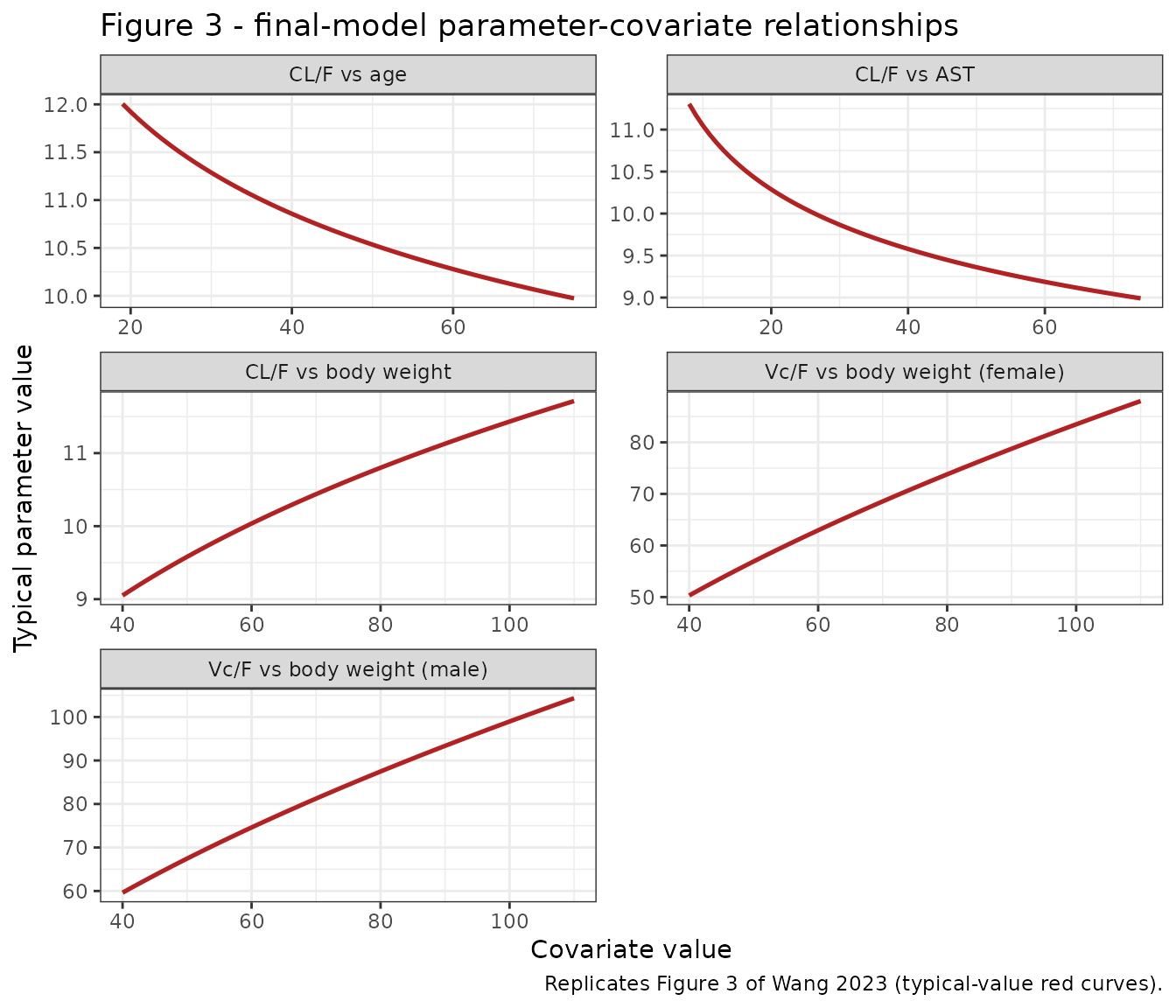

Cross-checking the endpoints of those curves against the percentage changes Wang 2023 quotes in its Discussion is an exact test of the four continuous coefficients:

disc <- tibble::tribble(
  ~Parameter, ~Covariate,          ~Simulated,                              ~`Wang 2023 Discussion`,
  "CL/F",     "WT 55 kg",          cl_typ(WT = 55) / cl_typ() - 1,          -0.0563,
  "CL/F",     "WT 83 kg",          cl_typ(WT = 83) / cl_typ() - 1,           0.0483,
  "Vc/F",     "WT 55 kg",          vc_typ(WT = 55) / vc_typ() - 1,          -0.1180,
  "Vc/F",     "WT 83 kg",          vc_typ(WT = 83) / vc_typ() - 1,           0.1080,
  "CL/F",     "AGE 41 y",          cl_typ(AGE = 41) / cl_typ() - 1,          0.0406,
  "CL/F",     "AGE 66 y",          cl_typ(AGE = 66) / cl_typ() - 1,         -0.0244,
  "CL/F",     "AST 13 U/L",        cl_typ(AST = 13) / cl_typ() - 1,          0.0341,
  "CL/F",     "AST 28 U/L",        cl_typ(AST = 28) / cl_typ() - 1,         -0.0445,
  "Vc/F",     "Female vs male",    vc_typ(SEXF = 1) / vc_typ() - 1,         -0.1570,
  "CL/F",     "Early-phase study", exp(0.203) - 1,                           0.2250
) |>
  dplyr::mutate(
    `Difference (pp)` = 100 * (Simulated - `Wang 2023 Discussion`),
    Simulated = sprintf("%+.2f%%", 100 * Simulated),
    `Wang 2023 Discussion` = sprintf("%+.2f%%", 100 * `Wang 2023 Discussion`)
  )

knitr::kable(disc, digits = 3,
             caption = "Parameter-level covariate effects vs the values quoted in the Wang 2023 Discussion.")

Parameter-level covariate effects vs the values quoted in the Wang 2023 Discussion.

Parameter	Covariate	Simulated	Wang 2023 Discussion	Difference (pp)
CL/F	WT 55 kg	-5.62%	-5.63%	0.011
CL/F	WT 83 kg	+4.82%	+4.83%	-0.007
Vc/F	WT 55 kg	-11.79%	-11.80%	0.014
Vc/F	WT 83 kg	+10.76%	+10.80%	-0.044
CL/F	AGE 41 y	+4.05%	+4.06%	-0.015
CL/F	AGE 66 y	-2.43%	-2.44%	0.009
CL/F	AST 13 U/L	+3.41%	+3.41%	-0.001
CL/F	AST 28 U/L	-4.45%	-4.45%	0.001
Vc/F	Female vs male	-15.63%	-15.70%	0.066
CL/F	Early-phase study	+22.51%	+22.50%	0.007

# Every coefficient must reproduce the paper's own percentage to within
# 0.1 percentage points (the paper rounds to 3 significant figures).
stopifnot(all(abs(disc$`Difference (pp)`) < 0.1))

Replicate Section 3.3 / Figure 4: sensitivity analysis

Wang 2023 Figure 4 is a tornado plot of the effect of each significant covariate on steady-state exposure in a typical subject after 10 repeated 75 mg twice-daily doses. Section 3.3 quotes the resulting percentage changes. For the three continuous covariates the paper reports a range, which turns out to be the minimum and maximum across the three exposure metrics (AUCtau,ss, Cmax,ss, Cmin,ss); for sex and meal timing it reports each metric separately.

Because each scenario perturbs a single covariate while holding the others at their population medians, this is exactly reproducible from the packaged model without needing the individual-level dataset.

scenarios <- tibble::tribble(
  ~scenario,              ~WT, ~AGE, ~AST, ~SEXF, ~STUDY_DORZA_EARLY, ~MEAL_DELAY_1H,
  "Typical (base)",        69,   55,   18,     0,                  0,              0,
  "WT 55 kg",              55,   55,   18,     0,                  0,              0,
  "WT 83 kg",              83,   55,   18,     0,                  0,              0,
  "AST 13 U/L",            69,   55,   13,     0,                  0,              0,
  "AST 28 U/L",            69,   55,   28,     0,                  0,              0,
  "AGE 41 y",              69,   41,   18,     0,                  0,              0,
  "AGE 66 y",              69,   66,   18,     0,                  0,              0,
  "Female",                69,   55,   18,     1,                  0,              0,
  "Meal >= 1 h post-dose", 69,   55,   18,     0,                  0,              1,
  "Early-phase study",     69,   55,   18,     0,                  1,              0
) |>
  dplyr::mutate(id = dplyr::row_number())

sens_events <- do.call(
  rbind,
  lapply(seq_len(nrow(scenarios)), function(i) {
    s <- scenarios[i, ]
    make_events(
      id = s$id, WT = s$WT, AGE = s$AGE, AST = s$AST, SEXF = s$SEXF,
      STUDY_DORZA_EARLY = s$STUDY_DORZA_EARLY,
      MEAL_DELAY_1H = s$MEAL_DELAY_1H, scenario = s$scenario
    )
  })
)
stopifnot(!anyDuplicated(unique(sens_events[, c("id", "time", "evid")])))

sim_sens <- rxode2::rxSolve(
  mod, sens_events, omega = NA, sigma = NA,
  keep = "scenario", returnType = "data.frame"
)

# Steady-state exposure metrics over the final dosing interval. AUCtau uses the
# linear trapezoidal rule, matching Wang 2023 Section 2.6 ("AUCtau,ss was
# calculated using the linear trapezoidal approximation"); the PKNCA section
# below independently confirms these numbers.
ss_metrics <- sim_sens |>
  dplyr::filter(time >= ss_start, time <= ss_end) |>
  dplyr::arrange(scenario, time) |>
  dplyr::group_by(scenario) |>
  dplyr::summarise(
    AUCtau = sum(diff(time) * (head(Cc, -1) + tail(Cc, -1)) / 2),
    Cmax   = max(Cc),
    Cmin   = min(Cc),
    .groups = "drop"
  )

base_ss <- ss_metrics |> dplyr::filter(scenario == "Typical (base)")

sens_pct <- ss_metrics |>
  dplyr::filter(scenario != "Typical (base)") |>
  dplyr::mutate(
    `AUCtau,ss` = 100 * (AUCtau / base_ss$AUCtau - 1),
    `Cmax,ss`   = 100 * (Cmax   / base_ss$Cmax   - 1),
    `Cmin,ss`   = 100 * (Cmin   / base_ss$Cmin   - 1)
  ) |>
  dplyr::select(scenario, `AUCtau,ss`, `Cmax,ss`, `Cmin,ss`)

sens_pct |>
  dplyr::rename("Scenario" = scenario) |>
  knitr::kable(
    digits = 2,
    caption = "Percent change in steady-state exposure vs the typical subject (75 mg BID, 10 doses). Replicates Figure 4 / Section 3.3 of Wang 2023."
  )

Percent change in steady-state exposure vs the typical subject (75 mg BID, 10 doses). Replicates Figure 4 / Section 3.3 of Wang 2023.

Scenario	AUCtau,ss	Cmax,ss	Cmin,ss
AGE 41 y	-3.89	-2.04	-6.81
AGE 66 y	2.49	1.31	4.40
AST 13 U/L	-3.29	-1.73	-5.77
AST 28 U/L	4.65	2.46	8.25
Early-phase study	-18.36	-9.55	-31.31
Female	0.01	9.03	-11.62
Meal >= 1 h post-dose	0.00	-1.30	2.71
WT 55 kg	5.95	9.60	1.60
WT 83 kg	-4.60	-7.09	-1.33

The paper’s reported values, and the assertions that pin them:

rng <- function(sc) {
  r <- sens_pct |> dplyr::filter(scenario == sc)
  c(min = min(c(r$`AUCtau,ss`, r$`Cmax,ss`, r$`Cmin,ss`)),
    max = max(c(r$`AUCtau,ss`, r$`Cmax,ss`, r$`Cmin,ss`)))
}

reported <- tibble::tribble(
  ~Scenario,               ~`Wang 2023 Section 3.3`,                ~`Simulated range`,
  "WT 55 kg",              "+1.63% to +9.62%",  sprintf("%+.2f%% to %+.2f%%", rng("WT 55 kg")[1], rng("WT 55 kg")[2]),
  "WT 83 kg",              "-7.1% to -1.35%",   sprintf("%+.2f%% to %+.2f%%", rng("WT 83 kg")[1], rng("WT 83 kg")[2]),
  "AST 13 U/L",            "-5.77% to -1.73%",  sprintf("%+.2f%% to %+.2f%%", rng("AST 13 U/L")[1], rng("AST 13 U/L")[2]),
  "AST 28 U/L",            "+2.45% to +8.24%",  sprintf("%+.2f%% to %+.2f%%", rng("AST 28 U/L")[1], rng("AST 28 U/L")[2]),
  "AGE 41 y",              "-6.82% to -2.04%",  sprintf("%+.2f%% to %+.2f%%", rng("AGE 41 y")[1], rng("AGE 41 y")[2]),
  "AGE 66 y",              "+1.31% to +4.41%",  sprintf("%+.2f%% to %+.2f%%", rng("AGE 66 y")[1], rng("AGE 66 y")[2]),
  "Female",                "AUCtau 0.01%, Cmax 9.09%, Cmin -11.6%",
                           sprintf("AUCtau %+.2f%%, Cmax %+.2f%%, Cmin %+.2f%%",
                                   sens_pct$`AUCtau,ss`[sens_pct$scenario == "Female"],
                                   sens_pct$`Cmax,ss`[sens_pct$scenario == "Female"],
                                   sens_pct$`Cmin,ss`[sens_pct$scenario == "Female"]),
  "Meal >= 1 h post-dose", "AUCtau no difference, Cmax -1.26%, Cmin 2.71%",
                           sprintf("AUCtau %+.2f%%, Cmax %+.2f%%, Cmin %+.2f%%",
                                   sens_pct$`AUCtau,ss`[sens_pct$scenario == "Meal >= 1 h post-dose"],
                                   sens_pct$`Cmax,ss`[sens_pct$scenario == "Meal >= 1 h post-dose"],
                                   sens_pct$`Cmin,ss`[sens_pct$scenario == "Meal >= 1 h post-dose"])
)
knitr::kable(reported,
             caption = "Simulated steady-state sensitivity vs the values reported in Wang 2023 Section 3.3.")

Simulated steady-state sensitivity vs the values reported in Wang 2023 Section 3.3.

Scenario	Wang 2023 Section 3.3	Simulated range
WT 55 kg	+1.63% to +9.62%	+1.60% to +9.60%
WT 83 kg	-7.1% to -1.35%	-7.09% to -1.33%
AST 13 U/L	-5.77% to -1.73%	-5.77% to -1.73%
AST 28 U/L	+2.45% to +8.24%	+2.46% to +8.25%
AGE 41 y	-6.82% to -2.04%	-6.81% to -2.04%
AGE 66 y	+1.31% to +4.41%	+1.31% to +4.40%
Female	AUCtau 0.01%, Cmax 9.09%, Cmin -11.6%	AUCtau +0.01%, Cmax +9.03%, Cmin -11.62%
Meal >= 1 h post-dose	AUCtau no difference, Cmax -1.26%, Cmin 2.71%	AUCtau -0.00%, Cmax -1.30%, Cmin +2.71%

# Continuous-covariate ranges: both endpoints within 0.1 percentage points.
stopifnot(
  abs(rng("WT 55 kg")   - c( 1.63,  9.62)) < 0.1,
  abs(rng("WT 83 kg")   - c(-7.10, -1.35)) < 0.1,
  abs(rng("AST 13 U/L") - c(-5.77, -1.73)) < 0.1,
  abs(rng("AST 28 U/L") - c( 2.45,  8.24)) < 0.1,
  abs(rng("AGE 41 y")   - c(-6.82, -2.04)) < 0.1,
  abs(rng("AGE 66 y")   - c( 1.31,  4.41)) < 0.1
)

# Sex and meal timing, per metric.
fem  <- sens_pct |> dplyr::filter(scenario == "Female")
meal <- sens_pct |> dplyr::filter(scenario == "Meal >= 1 h post-dose")
stopifnot(
  abs(fem$`AUCtau,ss` -   0.01) < 0.05,
  abs(fem$`Cmax,ss`   -   9.09) < 0.1,
  abs(fem$`Cmin,ss`   - (-11.6)) < 0.1,
  abs(meal$`Cmax,ss`  - (-1.26)) < 0.1,
  abs(meal$`Cmin,ss`  -   2.71)  < 0.05
)

Structural invariants

Two of the paper’s findings are exact structural consequences of where each covariate acts, and are therefore sharper tests than a tolerance band. Sex acts only on Vc/F and meal timing only on D1; neither touches CL/F, so steady-state AUCtau (which equals Dose / (CL/F) for a linear model) must be identically unchanged. Wang 2023 reports 0.01% and “no difference” respectively.

invariants <- tibble::tibble(
  Invariant = c("AUCtau,ss unchanged by sex (acts on Vc/F only)",
                "AUCtau,ss unchanged by meal timing (acts on D1 only)",
                "CL/F ratio, early-phase vs later-phase studies"),
  Simulated = c(sprintf("%+.4f%%", fem$`AUCtau,ss`),
                sprintf("%+.4f%%", meal$`AUCtau,ss`),
                sprintf("%.4f", exp(0.203))),
  Expected  = c("0% (Wang 2023 reports 0.01%)",
                "0% (Wang 2023 reports no difference)",
                "1.23 (Wang 2023 Table 3 CL_STUDY)")
)
knitr::kable(invariants, caption = "Structural invariants of the Wang 2023 covariate model.")

Structural invariants of the Wang 2023 covariate model.

Invariant	Simulated	Expected
AUCtau,ss unchanged by sex (acts on Vc/F only)	+0.0056%	0% (Wang 2023 reports 0.01%)
AUCtau,ss unchanged by meal timing (acts on D1 only)	-0.0003%	0% (Wang 2023 reports no difference)
CL/F ratio, early-phase vs later-phase studies	1.2251	1.23 (Wang 2023 Table 3 CL_STUDY)

# AUCtau is invariant to Vc/F and D1 up to ODE solver tolerance.
stopifnot(
  abs(fem$`AUCtau,ss`)  < 0.02,
  abs(meal$`AUCtau,ss`) < 0.02
)

Tornado plot

sens_pct |>
  tidyr::pivot_longer(-scenario, names_to = "metric", values_to = "pct") |>
  dplyr::mutate(
    metric = factor(metric, levels = c("AUCtau,ss", "Cmax,ss", "Cmin,ss"))
  ) |>
  ggplot(aes(pct, scenario)) +
  geom_col(fill = "steelblue") +
  geom_vline(xintercept = 0, linewidth = 0.4) +
  facet_wrap(~metric) +
  labs(
    x = "Change from typical subject (%)", y = NULL,
    title = "Figure 4 - covariate sensitivity on steady-state exposure",
    caption = "Replicates Figure 4 of Wang 2023 (75 mg BID, 10 doses, typical subject)."
  ) +
  theme_bw()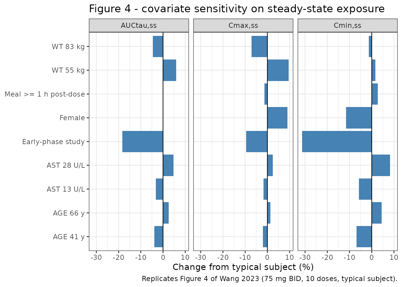

Dose linearity

Wang 2023 describes the model as a “two-compartment linear pharmacokinetic model”, and the first-in-human study reported dose-proportional exposure from 5 to 50 mg. Because nothing in the final model is dose- or concentration-dependent, steady-state exposure must scale exactly with dose. Pairing the dose arms turns this into a strict assertion rather than a visual check.

dose_levels <- c(25, 75, 200)

dose_events <- do.call(rbind, lapply(seq_along(dose_levels), function(i) {
  make_events(id = 100L + i, dose = dose_levels[i],
              scenario = paste0(dose_levels[i], " mg BID"))
}))
stopifnot(!anyDuplicated(unique(dose_events[, c("id", "time", "evid")])))

sim_dose <- rxode2::rxSolve(
  mod, dose_events, omega = NA, sigma = NA,
  keep = "scenario", returnType = "data.frame"
)

dose_lookup <- tibble::tibble(
  scenario = paste0(dose_levels, " mg BID"),
  dose     = dose_levels
)

dose_ss <- sim_dose |>
  dplyr::filter(time >= ss_start, time <= ss_end) |>
  dplyr::arrange(scenario, time) |>
  dplyr::group_by(scenario) |>
  dplyr::summarise(
    AUCtau = sum(diff(time) * (head(Cc, -1) + tail(Cc, -1)) / 2),
    Cmax   = max(Cc),
    .groups = "drop"
  ) |>
  dplyr::left_join(dose_lookup, by = "scenario") |>
  dplyr::mutate(
    `AUCtau/dose` = AUCtau / dose,
    `Cmax/dose`   = Cmax / dose
  )

dose_ss |>
  dplyr::select(-dose) |>
  dplyr::rename(
    "Regimen" = scenario,
    "AUCtau,ss (ng*h/mL)" = AUCtau,
    "Cmax,ss (ng/mL)" = Cmax,
    "AUCtau,ss per mg" = `AUCtau/dose`,
    "Cmax,ss per mg" = `Cmax/dose`
  ) |>
  knitr::kable(digits = 3,
               caption = "Dose-normalised steady-state exposure. A linear model gives identical values across dose levels.")

Dose-normalised steady-state exposure. A linear model gives identical values across dose levels.

Regimen	AUCtau,ss (ng*h/mL)	Cmax,ss (ng/mL)	AUCtau,ss per mg	Cmax,ss per mg
200 mg BID	19228.110	2806.728	96.141	14.034
25 mg BID	2403.514	350.841	96.141	14.034
75 mg BID	7210.541	1052.523	96.141	14.034

# Dose-normalised exposure is identical across arms to solver tolerance.
stopifnot(
  diff(range(dose_ss$`AUCtau/dose`)) / mean(dose_ss$`AUCtau/dose`) < 1e-6,
  diff(range(dose_ss$`Cmax/dose`))   / mean(dose_ss$`Cmax/dose`)   < 1e-6
)

Virtual cohort

Original observed data are not available. The cohort below is calibrated to the distributions Wang 2023 actually reports: the medians come from Table 2 (Overall column) and the dispersions are set so the 10th and 90th percentiles match the values quoted in the Discussion (WT 55 and 83 kg, AGE 41 and 66 years, AST 13 and 28 U/L about medians of 69 kg, 55 years and 18 U/L). Each covariate is drawn log-normal and truncated to the reported min-max range.

set.seed(20230803)
n_sub <- 200   # per-arm cap

# log-SD implied by median and the reported 10th / 90th percentiles
logsd <- function(p10, p90) (log(p90) - log(p10)) / (2 * stats::qnorm(0.9))

rtrunc_lnorm <- function(n, med, sd_log, lo, hi) {
  x <- stats::rlnorm(n, log(med), sd_log)
  pmin(pmax(x, lo), hi)
}

cohort <- tibble::tibble(
  id  = seq_len(n_sub),
  WT  = rtrunc_lnorm(n_sub, 69, logsd(55, 83), 40,  110),
  AGE = rtrunc_lnorm(n_sub, 55, logsd(41, 66), 19,  74.2),
  AST = rtrunc_lnorm(n_sub, 18, logsd(13, 28),  8,   74),
  SEXF = stats::rbinom(n_sub, 1, 0.374),          # Table 2: 397/1062 female
  # 83 of 1062 subjects (studies 102 / 103 / 110) carry the early-study effect
  STUDY_DORZA_EARLY = stats::rbinom(n_sub, 1, 83 / 1062),
  MEAL_DELAY_1H = 0                               # reference level; see Assumptions
)

cohort |>
  dplyr::summarise(
    `WT median` = stats::median(WT), `WT p10` = stats::quantile(WT, 0.1),
    `WT p90` = stats::quantile(WT, 0.9),
    `AGE median` = stats::median(AGE), `AST median` = stats::median(AST),
    `Female %` = 100 * mean(SEXF)
  ) |>
  knitr::kable(digits = 1,
               caption = "Virtual cohort covariate summary (target medians 69 kg / 55 y / 18 U/L, 37.4% female).")

Virtual cohort covariate summary (target medians 69 kg / 55 y / 18 U/L, 37.4% female).

WT median	WT p10	WT p90	AGE median	AST median	Female %
68.2	56.5	84.1	54.9	17.6	39.5

cohort_events <- do.call(rbind, lapply(seq_len(nrow(cohort)), function(i) {
  r <- cohort[i, ]
  make_events(
    id = r$id, WT = r$WT, AGE = r$AGE, AST = r$AST, SEXF = r$SEXF,
    STUDY_DORZA_EARLY = r$STUDY_DORZA_EARLY, MEAL_DELAY_1H = r$MEAL_DELAY_1H,
    scenario = "75 mg BID",
    times = sort(unique(c(seq(0, ss_start, by = 1), seq(ss_start, ss_end, by = 0.1))))
  )
}))
stopifnot(!anyDuplicated(unique(cohort_events[, c("id", "time", "evid")])))

Simulation

Inter-individual variability is retained; residual error is suppressed (sigma = NA) so the output is on the IPRED scale. This matches Wang 2023 Section 2.6, which simulated steady-state exposure “using the individual post-hoc parameter estimates” – i.e. individual predictions, not observations with residual noise. Comparing a residual-inflated Cmax against the paper’s post-hoc Cmax would bias the comparison upward.

sim_cohort <- rxode2::rxSolve(
  mod, cohort_events, sigma = NA,
  keep = "scenario", returnType = "data.frame"
)

sim_cohort |>
  dplyr::filter(time >= ss_start) |>
  dplyr::mutate(tad = time - ss_start) |>
  dplyr::group_by(tad) |>
  dplyr::summarise(
    Q025 = stats::quantile(Cc, 0.025),
    Q50  = stats::quantile(Cc, 0.500),
    Q975 = stats::quantile(Cc, 0.975),
    .groups = "drop"
  ) |>
  ggplot(aes(tad, Q50)) +
  geom_ribbon(aes(ymin = Q025, ymax = Q975), alpha = 0.25, fill = "steelblue") +
  geom_line(linewidth = 0.9) +
  labs(
    x = "Time after the 10th dose (h)", y = "Dorzagliatin (ng/mL)",
    title = "Steady-state concentration-time profile, 75 mg BID",
    caption = paste(
      "Median and 2.5th-97.5th percentile of", n_sub, "virtual subjects (IPRED scale).",
      "Illustrative analogue of the pooled prediction-corrected VPC in Figure 2 of Wang 2023."
    )
  ) +
  theme_bw()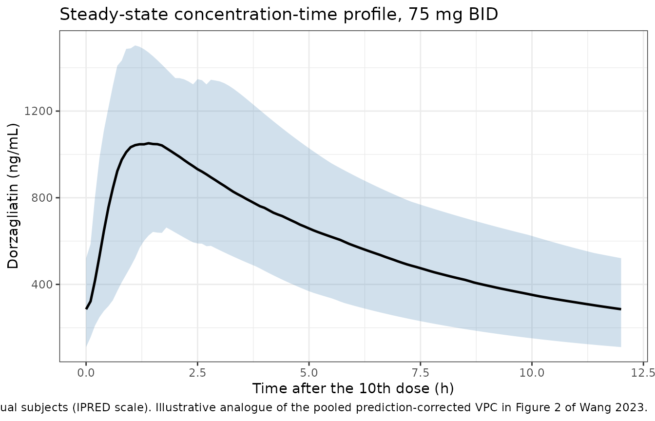

This is not a direct replication of Wang 2023 Figure 2: that figure is a prediction-corrected VPC pooling all six studies, all dose levels and all sampling schedules, which cannot be rebuilt without the original dataset. It is shown as an illustration of the model’s steady-state variability at the approved dose.

PKNCA validation

NCA is computed with PKNCA over the final dosing interval (108-120 h), the same window used for the exposure metrics above.

# Only `!is.na(Cc)` -- adding `time > 0` or `Cc > 0` would drop the time-zero
# row that PKNCA needs to anchor the AUC interval.
sim_nca <- sim_cohort |>
  dplyr::filter(!is.na(Cc)) |>
  dplyr::select(id, time, Cc, scenario)

# Guarantee a time = 0 row per subject; pre-dose Cc = 0 for an oral model.
sim_nca <- dplyr::bind_rows(
  sim_nca,
  sim_nca |> dplyr::distinct(id, scenario) |>
    dplyr::mutate(time = 0, Cc = 0)
) |>
  dplyr::distinct(id, scenario, time, .keep_all = TRUE) |>
  dplyr::arrange(id, scenario, time)

conc_obj <- PKNCA::PKNCAconc(
  sim_nca, Cc ~ time | scenario + id,
  concu = "ng/mL", timeu = "h"
)

dose_df <- cohort_events |>
  dplyr::filter(evid == 1) |>
  dplyr::select(id, time, amt, scenario)

dose_obj <- PKNCA::PKNCAdose(
  dose_df, amt ~ time | scenario + id, doseu = "mg"
)

intervals <- data.frame(
  start   = ss_start,
  end     = ss_end,
  cmax    = TRUE,
  tmax    = TRUE,
  cmin    = TRUE,
  auclast = TRUE,
  cav     = TRUE
)

nca_res <- PKNCA::pk.nca(
  PKNCA::PKNCAdata(conc_obj, dose_obj, intervals = intervals)
)

Comparison against published steady-state exposures

Wang 2023 Tables S1-S4 report geometric-mean steady-state exposures for the 75 mg twice-daily regimen. The overall-population values are recovered from Table S3, which gives both the normal-hepatic-function geometric mean and its percentage difference from the overall population: AUCtau,ss 7149 / (1 - 0.000526) = **7153 ng*h/mL, Cmax,ss 1089 / (1 + 0.00123) = 1088 ng/mL, and Cmin,ss 271 / (1 - 0.00319) = 272 ng/mL**.

ncaComparisonTable() summarises the simulated cohort by its median, which for a log-normally distributed exposure is the geometric mean – so the two sides of the table are on the same footing.

published <- tibble::tribble(
  ~scenario,    ~cmax, ~cmin, ~auclast,
  "75 mg BID",  1088,  272,   7153
)

cmp <- nlmixr2lib::ncaComparisonTable(
  simulated = nca_res,
  reference = published,
  by        = "scenario",
  units     = c(cmax = "ng/mL", cmin = "ng/mL", auclast = "ng*h/mL"),
  tolerance_pct = 20
)

knitr::kable(
  cmp,
  caption = "Simulated vs published steady-state exposure (75 mg BID). * differs from reference by >20%."
)

Simulated vs published steady-state exposure (75 mg BID). * differs from reference by >20%.

NCA parameter	scenario	Reference	Simulated	% diff
Cmax (ng/mL)	75 mg BID	1090	1090	+0.6%
Cmin (ng/mL)	75 mg BID	272	285	+4.8%
AUClast (ng*h/mL)	75 mg BID	7150	7180	+0.4%

The typical subject provides a second, exact anchor. For a linear model steady-state AUCtau equals Dose / (CL/F), so the simulated trapezoidal AUCtau must equal 75 mg / 10.4 L/h = 7212 ng*h/mL:

auc_analytic <- dose_mg / 10.4 * 1000     # mg / (L/h) -> ng*h/mL

anchor <- tibble::tibble(
  Quantity = c("AUCtau,ss, typical subject (simulated)",
               "AUCtau,ss, typical subject (analytic Dose / (CL/F))",
               "AUCtau,ss, overall population (Wang 2023 Table S3)"),
  Value = c(base_ss$AUCtau, auc_analytic, 7153)
)
anchor |>
  dplyr::rename("AUCtau,ss (ng*h/mL)" = Value) |>
  knitr::kable(digits = 1,
               caption = "Steady-state AUCtau anchors. The typical-subject simulation must equal Dose / (CL/F) exactly.")

Steady-state AUCtau anchors. The typical-subject simulation must equal Dose / (CL/F) exactly.

Quantity	AUCtau,ss (ng*h/mL)
AUCtau,ss, typical subject (simulated)	7210.5
AUCtau,ss, typical subject (analytic Dose / (CL/F))	7211.5
AUCtau,ss, overall population (Wang 2023 Table S3)	7153.0

stopifnot(abs(base_ss$AUCtau / auc_analytic - 1) < 0.001)

Half-life

The model’s analytic disposition half-lives follow from the Table 3 micro-constants. PKNCA’s half.life on a single-dose profile is compared against the analytic terminal (beta) half-life as an internal consistency check on the NCA step.

k10 <- 10.4 / 80.6
k12 <- 3.02 / 80.6
k21 <- 3.02 / 26.5
sm  <- k10 + k12 + k21
disc <- sqrt(sm^2 - 4 * k21 * k10)
t_half_alpha <- log(2) / (0.5 * (sm + disc))
t_half_beta  <- log(2) / (0.5 * (sm - disc))

# Single 75 mg dose, typical subject, sampled to 96 h.
sd_events <- make_events(
  id = 900L, doses = 0, scenario = "75 mg single dose",
  times = sort(unique(c(seq(0, 12, by = 0.05), seq(12, 96, by = 0.5))))
)
sim_sd <- rxode2::rxSolve(
  mod, sd_events, omega = NA, sigma = NA,
  keep = "scenario", returnType = "data.frame"
)

# rxSolve omits the `id` column when the solve has a single subject, so it is
# restored explicitly before handing the frame to PKNCA.
sd_nca <- sim_sd |>
  dplyr::filter(!is.na(Cc)) |>
  dplyr::mutate(id = 900L) |>
  dplyr::select(id, time, Cc, scenario)

sd_res <- PKNCA::pk.nca(PKNCA::PKNCAdata(
  PKNCA::PKNCAconc(sd_nca, Cc ~ time | scenario + id,
                   concu = "ng/mL", timeu = "h"),
  PKNCA::PKNCAdose(
    sd_events |> dplyr::filter(evid == 1) |>
      dplyr::select(id, time, amt, scenario),
    amt ~ time | scenario + id, doseu = "mg"
  ),
  intervals = data.frame(start = 0, end = Inf, cmax = TRUE, tmax = TRUE,
                         aucinf.obs = TRUE, half.life = TRUE)
))

nca_sd <- as.data.frame(sd_res)
t_half_nca <- nca_sd$PPORRES[nca_sd$PPTESTCD == "half.life"]

tibble::tibble(
  Quantity = c("Distribution half-life (alpha), analytic",
               "Terminal half-life (beta), analytic",
               "Terminal half-life, PKNCA on single-dose profile",
               "Reported NCA half-life range (Wang 2023 Introduction, ref. 7)"),
  `Value (h)` = c(sprintf("%.2f", t_half_alpha),
                  sprintf("%.2f", t_half_beta),
                  sprintf("%.2f", t_half_nca),
                  "4.5 - 8.6")
) |>
  knitr::kable(caption = "Dorzagliatin half-life from the packaged model vs the literature range cited by Wang 2023.")

Dorzagliatin half-life from the packaged model vs the literature range cited by Wang 2023.

Quantity	Value (h)
Distribution half-life (alpha), analytic	3.29
Terminal half-life (beta), analytic	9.93
Terminal half-life, PKNCA on single-dose profile	9.84
Reported NCA half-life range (Wang 2023 Introduction, ref. 7)	4.5 - 8.6

# PKNCA's lambda_z must recover the model's own analytic beta half-life.
stopifnot(abs(t_half_nca / t_half_beta - 1) < 0.05)

The analytic terminal half-life (9.9 h) sits above the 4.5-8.6 h range Wang 2023 quotes in its Introduction. That range comes from reference 7 (Miao 2022), a dedicated renal-impairment study whose NCA half-life was estimated from a finite sampling window (0-72 h) and is closer to an effective half-life than to the true terminal slope of a two-compartment model. The effective half-life implied by the accumulation this model predicts is the more comparable quantity:

first_int <- sim_typ |>
  dplyr::filter(time <= tau) |>
  dplyr::arrange(time)
auc_first <- sum(diff(first_int$time) *
                   (head(first_int$Cc, -1) + tail(first_int$Cc, -1)) / 2)
r_ac <- base_ss$AUCtau / auc_first
t_half_eff <- -tau * log(2) / log(1 - 1 / r_ac)

tibble::tibble(
  Quantity = c("AUCtau after the first dose (ng*h/mL)",
               "AUCtau at steady state (ng*h/mL)",
               "Accumulation ratio",
               "Effective half-life (h)"),
  Value = c(auc_first, base_ss$AUCtau, r_ac, t_half_eff)
) |>
  knitr::kable(digits = 2,
               caption = "Accumulation-derived effective half-life, the quantity most comparable to a windowed NCA half-life.")

Accumulation-derived effective half-life, the quantity most comparable to a windowed NCA half-life.

Quantity	Value
AUCtau after the first dose (ng*h/mL)	5066.32
AUCtau at steady state (ng*h/mL)	7210.54
Accumulation ratio	1.42
Effective half-life (h)	6.86

The effective half-life of 6.9 h falls inside the 4.5-8.6 h literature range, which reconciles the two figures: the packaged model is consistent with the reported half-life once the difference between a terminal-slope and an accumulation-based half-life is accounted for.

Assumptions and deviations

• Meal-timing covariate set to its reference level in the virtual cohort. Wang 2023 does not report how many subjects ate 0.5 h versus at least 1 h after dosing, so MEAL_DELAY_1H = 0 (the reference, eat at 0.5 h) is used for the cohort. The covariate acts only on D1, so this choice does not affect AUCtau,ss and shifts Cmax,ss / Cmin,ss by at most 1.3% / 2.7% (shown in the sensitivity section). Downstream users modelling a delayed-meal population should set the column to 1.
• Virtual-cohort covariate dispersions are inferred, not published. Table 2 reports median and min-max only. Log-normal dispersions were back-solved from the 10th and 90th percentiles the Discussion quotes (WT 55 / 83 kg, AGE 41 / 66 years, AST 13 / 28 U/L), then truncated to the Table 2 ranges. The covariates are drawn independently, whereas the real cohort has correlated demographics.
• Table S1, S2 and S4 subgroup differences are not reproduced. Those supplement tables compare exposure across BMI quartiles, age groups (< 65 vs >= 65 years) and renal-function groups using post-hoc individual parameter estimates on the actual 1062-subject covariate distribution. Wang 2023 states explicitly that “this simulation accounts for potential correlations among covariates” and that “the above differences also included the confounding effects of multiple factors”. The reported +9.11% AUCtau difference for age >= 65, for instance, is larger than the pure age coefficient predicts (about +3.4% for a 53 -> 68 year shift), because older subjects also differ in weight and AST. Reproducing those tables requires the individual-level dataset, which is available only from the corresponding author. The overall-population values (Table S3, recovered above) are reproduced instead.
• Renal function carries no effect in the model. Serum creatinine and creatinine clearance were screened and dropped, so the Table S4 renal-function differences arise entirely from correlated covariates. This matches the paper’s conclusion that no dose adjustment is needed at any stage of renal impairment (geometric mean ratio of ESRD to healthy volunteers 0.81 for Cmax and 1.11 for AUC, from reference 7).
• IIV reported as “approximate CV%”. Wang 2023 Table 3’s footnote reads “IIV for CL, Vc, Vp, D1, and proportional error are reported as approximate CV%”. The model reads this as the square-root-of-variance convention (omega = CV / 100) rather than the exact log-normal CV = sqrt(exp(omega^2) - 1), because only the former is an approximation. The two readings differ negligibly at these magnitudes (omega_CL 0.2250 vs 0.2222).
• Residual error suppressed for the exposure comparison. The cohort is simulated with sigma = NA so results are on the IPRED scale, matching Wang 2023 Section 2.6’s use of post-hoc individual parameter estimates. Including the 32.9% proportional plus 109 ng/mL additive residual error would inflate simulated Cmax,ss relative to the paper’s values.
• No IIV on ka or Q/F. Wang 2023 Table 3 reports IIV only for CL/F, Vc/F, Vp/F and D1. No variability is invented for the remaining parameters.
• Bioavailability is not a parameter. Only oral data were analysed, so all disposition parameters are apparent (/F) and F is implicitly 1. The between-study exposure difference that would ordinarily be modelled on F was instead absorbed into CL/F – see the errata note below.

Errata and source-document issues

These are transcription problems in the published article; the values used in the model file follow the printed equations, which are internally consistent with the paper’s own reported percentage changes.

• Table 3 mislabels the D1,FOOD row as “Influence of food consumption time on CL/F”. The printed equation places the effect on D1 (D1 = 0.418 * exp(0.816 * FOOD + eta_D1)), the parameter name is D1,FOOD, and the Discussion confirms “patients with time to food consumption of >= 1 h after drug administration had higher D1”. The model applies it to D1.
• Table 3’s “shrinkage” footnote duplicates the IIV column. It reads “The shrinkage of CL/F, Vc/F, Vp/F and D1 are 22.5%, 14.9%, 48.8% and 82.8%” – exactly the four IIV CV% values from the table body. These are the IIV estimates, not shrinkage; no shrinkage values are recoverable from the article.
• Supplement Table S2 and S4 row labels are wrong. In both tables the second and third exposure rows are labelled “Cmax,ss (ug/mL)” and “Cmax,ss (ng/mL)”; from the magnitudes and the accompanying main-text narrative these are Cmax,ss (ng/mL) and Cmin,ss (ng/mL). Table S4’s column headers additionally read “Normal / Mild Hepatic function” although its title and footnote both describe renal function groups.
• The female Vc effect is quoted three ways that do not round to each other. The printed equation coefficient is -0.170, Table 3 tabulates Vc,GEND = 0.843, and the Discussion says females are “15.7% lower”. But exp(-0.170) = 0.84366, which rounds to 0.844, not 0.843; conversely log(0.843) = -0.170788. Both printed numbers are roundings of the same underlying estimate (about -0.1708), at different precisions and on different scales. The model file uses the equation coefficient -0.170, per the convention that the printed equation governs. The practical consequence is negligible but was measured rather than assumed: -0.170 gives a female Vc/F 15.63% lower than male (vs the quoted 15.7%) and reproduces the paper’s Section 3.3 female Cmax,ss / Cmin,ss changes as +9.03% / -11.62% against the reported +9.09% / -11.6%. Using log(0.843) = -0.170788 instead reproduces the 15.7% and the +9.09% Cmax exactly but shifts Cmin,ss to -11.67%, so neither reading matches all three reported figures. Every difference is under 0.07 percentage points. Downstream users who need to match the paper’s Vc/F ratio exactly should override e_sexf_vc to log(0.843).
• Study-effect magnitude is quoted two ways. Table 3 gives CL_STUDY = 1.23 (three significant figures) while the Discussion says CL was “22.5% higher” in studies 102/103/110. The printed equation coefficient 0.203 reconciles them: exp(0.203) = 1.2251, i.e. 22.5% higher, rounding to 1.23 in the table. The model stores the log-scale 0.203.
• The between-study effect is mechanistically a bioavailability difference. Wang 2023 Discussion attributes the lower exposure in studies 102/103/110 to formulation (studies 301/302 used near-commercial preparations) but reports that “the model was unable to correct for prediction bias by bioavailability” in the sparsely-sampled later studies, so the difference was carried on CL/F. The covariate is therefore registered as STUDY_DORZA_EARLY (a study indicator) rather than as a formulation indicator: the formulation attribution is the paper’s hypothesis, not its parameterisation.