FAP-4-1BBL (RO7122290) + cibisatamab trimeric-complex dose selection (Sanchez 2023)
Source:vignettes/articles/Sanchez_2023_ro7122290_cibisatamab.Rmd
Sanchez_2023_ro7122290_cibisatamab.RmdModel and source
Sanchez et al. (2023) built a model-based workflow that starts from in vitro co-culture data and ends with a recommended clinical dose range for FAP-4-1BBL (RO7122290), a bispecific fusion protein that costimulates T cells through 4-1BB only while it is simultaneously bound to fibroblast activation protein (FAP) on cancer-associated fibroblasts. FAP-4-1BBL is given with the CEA x CD3 T-cell bispecific cibisatamab, which induces the 4-1BB that FAP-4-1BBL engages. The paper deposits Monolix code for its Model 1 and two RxODE scripts for the clinical simulations, and the three packaged models follow that split:
| Model file | What it holds | Paper section |
|---|---|---|
Sanchez_2023_ro7122290_invitro |
In vitro co-culture: Model 1 (4-1BB time course, mixed-effects fit), FAP-4-1BBL binding in the well, Model 3 (fold increase in killing), Model 2 (FAP-dependent loss of monotherapy killing) | Models 1-3, Figures 1-3 |
Sanchez_2023_ro7122290_qsp |
Clinical dose selection with 4-1BB held at 80 receptors per T cell | Simulation 1, Figure 4 |
Sanchez_2023_ro7122290_cibisatamab_qsp |
Clinical combination with cibisatamab PK, cibisatamab-driven 4-1BB (Model 1) and Models 2-3 in the tumor | Simulations 2-3, Figures 5-6 |
ui_vitro <- rxode2::rxode(readModelDb("Sanchez_2023_ro7122290_invitro"))
#> ℹ parameter labels from comments will be replaced by 'label()'
ui_dose <- rxode2::rxode(readModelDb("Sanchez_2023_ro7122290_qsp"))
#> ℹ parameter labels from comments will be replaced by 'label()'
ui_combo <- rxode2::rxode(readModelDb("Sanchez_2023_ro7122290_cibisatamab_qsp"))
#> ℹ parameter labels from comments will be replaced by 'label()'- Citation: Sanchez J, Claus C, Albrecht R, Gaillard BC, Marinho J, McIntyre C, Tanos T, Boehnke A, Friberg LE, Jonsson S, Frances N. A model-based approach leveraging in vitro data to support dose selection from the outset: A framework for bispecific antibodies in immuno-oncology. CPT Pharmacometrics Syst Pharmacol. 2023;12(11):1804-1818. doi:10.1002/psp4.13065
- Article: https://doi.org/10.1002/psp4.13065
- Supplementary information (Supplementary Materials and Methods, Table S1, Monolix and RxODE code): Data S1 of the article.
Population
No patients were fitted. The pharmacodynamics come from three in vitro experiments in which MKN-45 gastric cancer cells (high CEACAM5) were co-cultured with human PBMC effector cells at an effector:target ratio of 1:1 and with fibroblasts expressing FAP (Supplementary Materials and Methods):
- Experiment 1 (Model 1): cibisatamab 0, 0.2, 2, 20, 200 and 2000 nM, or 20 nM with 1 nM FAP-4-1BBL, fibroblasts at 92,000 FAP/fibroblast; 4-1BB per CD8+ T cell measured at 4, 21, 45 and 69 h.
- Experiment 2 (Model 3): 2 nM cibisatamab with FAP-4-1BBL 0 to 10,000 nM, fibroblasts at 92,000 (high) or 12,700 (low) FAP/fibroblast; tumor cell killing imaged for up to 138 h.
- Experiment 3 (Model 2): 0.2 nM cibisatamab with 0 to 100% of the fibroblasts expressing 6,800 FAP/fibroblast.
The clinical simulations use virtual colorectal carcinoma patients: the FAP-4-1BBL population PK of Micallef et al. (ACoP 2020) and an internal cibisatamab PK model, both tabulated in Table S1, with FAP expression from published immunohistochemistry H-scores (median 12% FAP-positive fibroblasts, 12,000 FAP/fibroblast).
str(ui_combo$population)
#> List of 6
#>  $ species      : chr "human (virtual patients; pharmacodynamics translated from in vitro co-culture data)"
#>  $ n_subjects   : int NA
#>  $ n_studies    : int NA
#>  $ disease_state: chr "Colorectal carcinoma (virtual patients); FAP expression from published immunohistochemistry H-scores"
#>  $ dose_range   : chr "Cibisatamab 100 mg q3w 2-h IV infusion followed by FAP-4-1BBL 1-180 mg 2-h IV infusion q1w, q2w or q3w"
#>  $ notes        : chr "No patients were fitted. FAP-4-1BBL population PK comes from Micallef et al. (ACoP 2020) and cibisatamab PK fro"| __truncated__
Source trace
Every ini() value carries a trailing comment naming its
source. Summary:
| Quantity | Value | Source |
|---|---|---|
lemax, lec50, lhill
|
537.682 receptors/cell, 16.004 nM, 0.210 | Table 2; Table S1 for the extra decimals |
lsignal2, lt_stop
|
381.92 receptors/cell, 16.18 h | Table 2; Table S1 |
lktr, lkin, lkout
|
0.2801 1/h, 2.952 receptors/cell/h, 0.2832 1/h | Table 2; Table S1 |
| Model 1 random effects | SD 0.1 held constant; SD 0.09 on ktr
|
Table 2 |
addSd |
5.36 receptors/cell | Table 2 |
kill_max, trimer50,
hill_kill, kill_base
|
4.37, 3.91e-3, 1.16, 1.04 | Table 3 (Model 3) |
kill_nofap, kill_maxdec,
hill_fap, logit_fap50
|
101.9%, 67.4%, 0.86, -1.1 | Table 3 (Model 2) |
kd_fap, koff_fap, kd_41bb,
koff_41bb
|
0.7 nM, 0.1 1/h, 0.2 nM, 0.1 1/h | Table S1 (kon = koff / KD) |
FAP-4-1BBL lvc, lvp, lcl,
lq
|
3.77 L, 0.83 L, 0.0154 L/h, 0.0219 L/h | Table S1 (volumes in mL in the deposited code) |
FAP-4-1BBL lvmax, lkm
|
0.455 mg/h, 5.18 mg/L | Table S1; mg/h from the deposited code (see Assumptions) |
| FAP-4-1BBL IIV | V1-CL block (0.485, 0.04, 0.104); V2 1.52; Vmax-Km block (0.306, 0.365, 0.798) | Deposited dose-selection code |
Cibisatamab lvc_, lvp_, lcl_,
lq_cibisatamab
|
3.95 L, 4.38 L, 0.063 L/h, 0.039 L/h | Table S1 |
ktum_in, ktum_out
|
0.06, 0.137 1/h (2.2:1); 0.03, 0.3 1/h (10:1) | Table S1 |
mw, mw_cibisatamab
|
177,000 and 194,000 g/mol | Deposited code (/0.177, *5.1546) |
| Tumor geometry, cell density, fibroblast fraction, E:T, T-cell fraction | 50 mm ellipsoid, 1e7 cells/cm^3, 0.15, 0.1, 40% x 0.4 | Deposited RxODE code |
fap_per_fib, fap_pos_pct (clinic) |
12,000, 12% | Supplementary Materials and Methods, Simulation 1 |
r41bb_tcell |
80 receptors per T cell | Supplementary Materials and Methods, Simulation 1 |
| Step function, Signal, transit chain, 4-1BB turnover | Equations 1-8 and 10-16 | Results, Model 1 and Model 3 |
| Binding ODEs and FAP initial condition | Equations 17-22 | Results, Model 3 |
| Receptor occupancy and trimers per cell | Equations 23-26 | Results, Model 3 |
| Fold increase in killing; monotherapy killing | Equations 27 and 9 | Results, Models 3 and 2 |
Model 1: 4-1BB expression on CD8+ T cells in vitro
Typical-value 4-1BB trajectories for every Experiment 1 condition, overlaid on the observed medians read off the individual-fit panels of Figure S4 by the maintainers.
conds <- tibble(
  cond = c("No TCB", "0.2 nM", "2 nM", "20 nM", "20 nM + FAP-4-1BBL 1 nM", "200 nM", "2000 nM"),
  cibi = c(0, 0.2, 2, 20, 20, 200, 2000),
  fap41bbl = c(0, 0, 0, 0, 1, 0, 0)
) |>
  mutate(id = row_number())

ev_m1 <- bind_rows(
  conds |> filter(fap41bbl > 0) |>
    transmute(id, time = 0, amt = fap41bbl, evid = 1, cmt = "medium"),
  conds |> tidyr::crossing(time = seq(0, 72, by = 1)) |>
    transmute(id, time, amt = 0, evid = 0, cmt = "expr_41bb")
) |>
  left_join(conds |> select(id, CONC_CIBISATAMAB_NM = cibi), by = "id") |>
  arrange(id, time, desc(evid))

sim_m1 <- rxSolve(rxode2::zeroRe(ui_vitro), ev_m1, returnType = "data.frame") |>
  left_join(conds |> select(id, cond), by = "id")
#> ℹ omega/sigma items treated as zero: 'etalemax', 'etalec50', 'etalhill', 'etalsignal2', 'etalt_stop', 'etalktr', 'etalkin', 'etalkout'
#> Warning: multi-subject simulation without without 'omega'

obs_m1 <- tribble(
  ~cond, ~time, ~obs,
  "No TCB", 4, 16.3, "No TCB", 21, 8.2, "No TCB", 45, 23.8, "No TCB", 69, -1,
  "0.2 nM", 4, 9.5, "0.2 nM", 21, 27.5, "0.2 nM", 45, 67.5, "0.2 nM", 69, 0.8,
  "2 nM", 4, 10, "2 nM", 21, 64.5, "2 nM", 45, 63, "2 nM", 69, 0.5,
  "20 nM", 4, 14, "20 nM", 21, 56, "20 nM", 45, 107, "20 nM", 69, 7,
  "20 nM + FAP-4-1BBL 1 nM", 4, 14, "20 nM + FAP-4-1BBL 1 nM", 21, 93,
  "20 nM + FAP-4-1BBL 1 nM", 45, 143, "20 nM + FAP-4-1BBL 1 nM", 69, 17,
  "200 nM", 4, 9, "200 nM", 21, 141, "200 nM", 45, 89, "200 nM", 69, 3,
  "2000 nM", 4, 10, "2000 nM", 21, 71, "2000 nM", 45, 173, "2000 nM", 69, 1
)

ggplot(sim_m1, aes(time, expr_41bb)) +
  geom_line(colour = "purple") +
  geom_point(data = obs_m1, aes(time, obs), colour = "steelblue") +
  facet_wrap(~ factor(cond, levels = conds$cond), scales = "free_y") +
  labs(x = "Time (h)", y = "4-1BB receptors per CD8+ T cell",
       caption = "Typical-value predictions; points read off Figure S4 of Sanchez 2023.")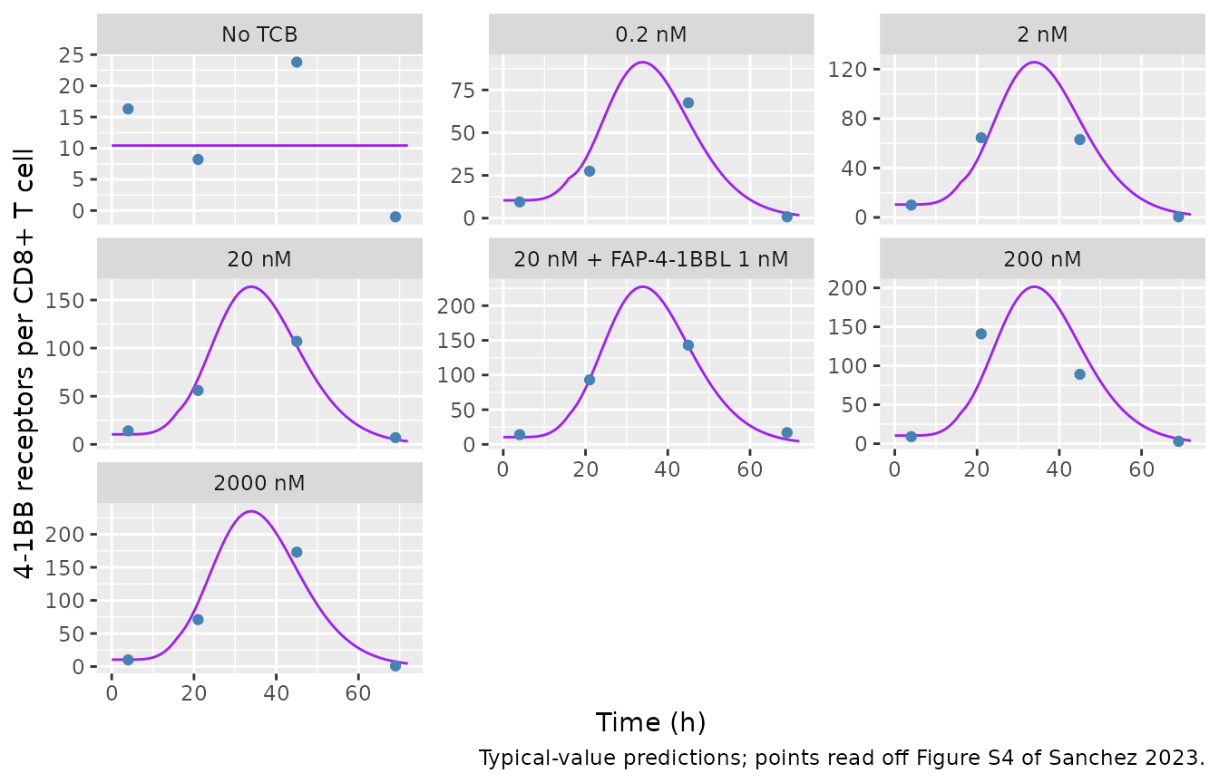
m1_cmp <- obs_m1 |>
  filter(time %in% c(21, 45), cond != "No TCB") |>
  left_join(sim_m1 |> select(cond, time, pred = expr_41bb), by = c("cond", "time"))
knitr::kable(m1_cmp, digits = 1)| cond | time | obs | pred |
|---|---|---|---|
| 0.2 nM | 21 | 27.5 | 39.2 |
| 0.2 nM | 45 | 67.5 | 56.9 |
| 2 nM | 21 | 64.5 | 53.0 |
| 2 nM | 45 | 63.0 | 78.4 |
| 20 nM | 21 | 56.0 | 68.2 |
| 20 nM | 45 | 107.0 | 102.2 |
| 20 nM + FAP-4-1BBL 1 nM | 21 | 93.0 | 93.7 |
| 20 nM + FAP-4-1BBL 1 nM | 45 | 143.0 | 141.9 |
| 200 nM | 21 | 141.0 | 83.3 |
| 200 nM | 45 | 89.0 | 125.8 |
| 2000 nM | 21 | 71.0 | 96.7 |
| 2000 nM | 45 | 173.0 | 146.6 |
# The combination condition is fitted through Signal2, which is 39% above the
# monotherapy Signal at the same 20 nM cibisatamab.
sig_ratio <- exp(ui_vitro$theta["lsignal2"]) /
  (exp(ui_vitro$theta["lemax"]) * 20^exp(ui_vitro$theta["lhill"]) /
     (20^exp(ui_vitro$theta["lhill"]) + exp(ui_vitro$theta["lec50"])^exp(ui_vitro$theta["lhill"])))
sig_ratio
#> lsignal2
#> 1.388135
stopifnot(
  abs(sig_ratio - 1.39) < 0.01,
  # Typical predictions sit within the individual-fit scatter of the medians.
  median(abs(m1_cmp$pred - m1_cmp$obs) / m1_cmp$obs) < 0.35
)
Model 3: trimeric complexes and tumor cell killing in vitro
Experiment 2 conditions: 2 nM cibisatamab, 10,000 fibroblasts in 200 uL, and FAP-4-1BBL added at time zero. The trimeric complexes per T cell are averaged over 0-120 h before entering the Emax model (Equation 27).
grid <- tidyr::expand_grid(
  fap_per_fib = 10^seq(2, log10(5e5), length.out = 30),
  conc = 10^seq(-3, 3, length.out = 31)
) |>
  mutate(id = row_number())

ev_grid <- bind_rows(
  grid |> transmute(id, time = 0, amt = conc, evid = 1, cmt = "medium"),
  grid |> transmute(id, time = 120, amt = 0, evid = 0, cmt = "trimer")
) |>
  mutate(CONC_CIBISATAMAB_NM = 2) |>
  arrange(id, time, desc(evid))

sim_grid <- rxSolve(
  rxode2::zeroRe(ui_vitro), ev_grid,
  params = grid |> select(id, fap_per_fib),
  returnType = "data.frame"
) |>
  select(id, trimer_avg) |>
  left_join(grid, by = "id")
#> ℹ omega/sigma items treated as zero: 'etalemax', 'etalec50', 'etalhill', 'etalsignal2', 'etalt_stop', 'etalktr', 'etalkin', 'etalkout'
#> Warning: multi-subject simulation without without 'omega'

ggplot(sim_grid, aes(fap_per_fib, conc, fill = log10(trimer_avg))) +
  geom_raster(interpolate = TRUE) +
  geom_contour(aes(z = trimer_avg), breaks = 2.6e-2, colour = "red") +
  geom_vline(xintercept = 13400, linetype = "dashed") +
  scale_x_log10() + scale_y_log10() +
  scale_fill_viridis_c(option = "plasma") +
  labs(x = "FAP per fibroblast", y = "FAP-4-1BBL (nM)", fill = "log10 trimers\nper T cell",
       caption = "Replicates Figure 3c of Sanchez 2023; red contour = 2.6e-2 trimeric complexes per T cell.")
#> Warning: The following aesthetics were dropped during statistical transformation: fill.
#> ℹ This can happen when ggplot fails to infer the correct grouping structure in
#>   the data.
#> ℹ Did you forget to specify a `group` aesthetic or to convert a numerical
#>   variable into a factor?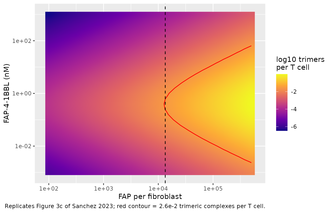
The paper quotes three points on the 2.6e-2 contour (90% of the maximum fold increase): the minimum of 13,400 FAP/fibroblast reached only at 0.37 nM, and the range 0.01-11.5 nM at 100,000 FAP/fibroblast.
fig3c <- tibble(
  fap_per_fib = c(13400, 1e5, 1e5),
  conc = c(0.37, 0.0115, 11.5),
  id = 1:3
)
ev3 <- bind_rows(
  fig3c |> transmute(id, time = 0, amt = conc, evid = 1, cmt = "medium"),
  fig3c |> transmute(id, time = 120, amt = 0, evid = 0, cmt = "trimer")
) |>
  mutate(CONC_CIBISATAMAB_NM = 2) |>
  arrange(id, time, desc(evid))
pts <- rxSolve(rxode2::zeroRe(ui_vitro), ev3, params = fig3c |> select(id, fap_per_fib),
               returnType = "data.frame") |>
  select(id, trimer_avg) |>
  left_join(fig3c, by = "id") |>
  mutate(published = 2.6e-2, pct_diff = 100 * (trimer_avg / published - 1))
#> ℹ omega/sigma items treated as zero: 'etalemax', 'etalec50', 'etalhill', 'etalsignal2', 'etalt_stop', 'etalktr', 'etalkin', 'etalkout'
#> Warning: multi-subject simulation without without 'omega'
pts |>
  select(fap_per_fib, conc, trimer_avg, published, pct_diff) |>
  dplyr::rename("FAP per fibroblast" = fap_per_fib, "FAP-4-1BBL (nM)" = conc,
                "Simulated trimers per T cell" = trimer_avg,
                "Figure 3c" = published, "% difference" = pct_diff) |>
knitr::kable(digits = 4)| FAP per fibroblast | FAP-4-1BBL (nM) | Simulated trimers per T cell | Figure 3c | % difference |
|---|---|---|---|---|
| 13400 | 0.3700 | 0.0271 | 0.026 | 4.1386 |
| 100000 | 0.0115 | 0.0248 | 0.026 | -4.4451 |
| 100000 | 11.5000 | 0.0273 | 0.026 | 4.8201 |
# Deterministic typical-value solve: the binding constants, Model 1 and the
# Signal2/Signal ratio fix these values exactly.
stopifnot(all(abs(pts$pct_diff) < 10))
Fold increase in killing over the Experiment 2 concentration range (the bell shape of Figure 3a, observed means read off the figure by the maintainers):
bell <- tidyr::expand_grid(
  fap = c(High = 92000, Low = 12700),
  conc = c(0, 0.01, 0.1, 1, 10, 100, 1000, 10000)
) |>
  mutate(level = rep(c("High FAP", "Low FAP"), each = 8), id = row_number())
ev_bell <- bind_rows(
  bell |> filter(conc > 0) |> transmute(id, time = 0, amt = conc, evid = 1, cmt = "medium"),
  bell |> transmute(id, time = 120, amt = 0, evid = 0, cmt = "trimer")
) |>
  mutate(CONC_CIBISATAMAB_NM = 2) |>
  arrange(id, time, desc(evid))
sim_bell <- rxSolve(rxode2::zeroRe(ui_vitro), ev_bell,
                    params = bell |> select(id, fap_per_fib = fap),
                    returnType = "data.frame") |>
  select(id, fold_kill) |>
  left_join(bell |> select(id, level, conc), by = "id") |>
  mutate(obs = c(1.0, 3.8, 4.2, 4.3, 4.45, 2.45, 1.45, 1.0,
                 1.05, 2.0, 3.75, 4.1, 2.45, 1.6, 1.15, 1.0))
#> ℹ omega/sigma items treated as zero: 'etalemax', 'etalec50', 'etalhill', 'etalsignal2', 'etalt_stop', 'etalktr', 'etalkin', 'etalkout'
#> Warning: multi-subject simulation without without 'omega'
ggplot(sim_bell, aes(pmax(conc, 1e-3), fold_kill, colour = level)) +
  geom_line() + geom_point(aes(y = obs), shape = 1, size = 2) +
  scale_x_log10() +
  labs(x = "FAP-4-1BBL (nM; 0 plotted at 1e-3)", y = "Fold increase vs cibisatamab alone",
       caption = "Lines: model at 120 h; open circles: means read off Figure 3a.")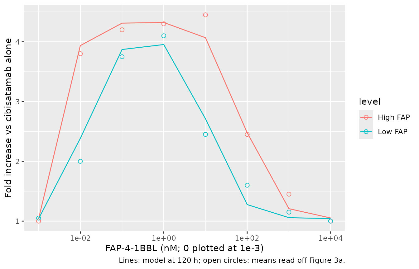
Model 2: cibisatamab monotherapy killing versus FAP-positive fibroblasts
m2 <- tibble(fap_pos_pct = c(0, 5, 10, 15, 20, 40, 60, 100), id = seq_len(8))
ev_m2 <- m2 |>
  transmute(id, time = 0, amt = 0, evid = 0, cmt = "trimer", CONC_CIBISATAMAB_NM = 0.2)
sim_m2 <- rxSolve(rxode2::zeroRe(ui_vitro), ev_m2, params = m2, returnType = "data.frame") |>
  select(id, kill_mono_pct) |>
  left_join(m2, by = "id")
#> ℹ omega/sigma items treated as zero: 'etalemax', 'etalec50', 'etalhill', 'etalsignal2', 'etalt_stop', 'etalktr', 'etalkin', 'etalkout'
#> Warning: multi-subject simulation without without 'omega'
sim_m2 |>
  select(fap_pos_pct, kill_mono_pct) |>
  dplyr::rename("FAP-positive fibroblasts (%)" = fap_pos_pct,
                "Monotherapy killing (% of 0% FAP)" = kill_mono_pct) |>
knitr::kable(digits = 1)| FAP-positive fibroblasts (%) | Monotherapy killing (% of 0% FAP) |
|---|---|
| 0 | 101.5 |
| 5 | 90.4 |
| 10 | 83.0 |
| 15 | 77.2 |
| 20 | 72.3 |
| 40 | 58.4 |
| 60 | 49.0 |
| 100 | 34.6 |
Simulation 1: dose selection for maximum trimeric complex formation
Area under the trimeric-complex curve (trimer_per_tcell)
over 30 weeks of FAP-4-1BBL infused over 2 h q1w, q2w or q3w, for 100
virtual patients with IIV on the FAP-4-1BBL PK only, under the 2.2:1 and
10:1 plasma:tumor distribution scenarios. The same 100 random-effect
draws are reused at every dose so the dose-response curve is not
confounded by resampling.
set.seed(20231)
n_pat <- 100
om <- ui_dose$omega
draws <- matrix(rnorm(n_pat * nrow(om)), n_pat) %*% chol(om)
colnames(draws) <- colnames(om)
draws <- as.data.frame(draws)

doses <- c(1, 2, 3, 5, 7, 10, 14, 21, 30, 45, 67, 100, 145)
scen <- tibble(
  scenario = c("2.2:1", "10:1"),
  ktum_in = c(0.06, 0.03),
  ktum_out = c(0.137, 0.3)
)
t_end <- 24 * 7 * 30
trap <- function(x, y) sum(diff(x) * (head(y, -1) + tail(y, -1)) / 2)

auc_one <- function(dose, weeks, s) {
  ev <- rxode2::et(amt = dose, rate = dose / 2, ii = weeks * 168,
                   until = t_end - 1, cmt = "central") |>
    rxode2::et(seq(0, t_end, by = 2))
  prm <- cbind(draws, ktum_in = s$ktum_in, ktum_out = s$ktum_out)
  # One shared event table with one params row per patient: rxSolve labels
  # the patients `sim.id`.
  out <- rxSolve(rxode2::zeroRe(ui_dose), ev, params = prm, returnType = "data.frame")
  out |>
    group_by(id = sim.id) |>
    summarise(auc = trap(time, trimer_per_tcell), .groups = "drop") |>
    mutate(dose = dose, schedule = paste0("q", weeks, "w"), scenario = s$scenario)
}

sim1 <- bind_rows(lapply(seq_len(nrow(scen)), function(i) {
  bind_rows(lapply(1:3, function(w) bind_rows(lapply(doses, auc_one, weeks = w, s = scen[i, ]))))
}))
#> Warning: No sigma parameters in the model
#> No sigma parameters in the model
#> No sigma parameters in the model
#> No sigma parameters in the model
#> No sigma parameters in the model
#> No sigma parameters in the model
#> No sigma parameters in the model
#> No sigma parameters in the model
#> No sigma parameters in the model
#> No sigma parameters in the model
#> No sigma parameters in the model
#> No sigma parameters in the model
#> No sigma parameters in the model
#> No sigma parameters in the model
#> No sigma parameters in the model
#> No sigma parameters in the model
#> No sigma parameters in the model
#> No sigma parameters in the model
#> No sigma parameters in the model
#> No sigma parameters in the model
#> No sigma parameters in the model
#> No sigma parameters in the model
#> No sigma parameters in the model
#> No sigma parameters in the model
#> No sigma parameters in the model
#> No sigma parameters in the model
#> No sigma parameters in the model
#> No sigma parameters in the model
#> No sigma parameters in the model
#> No sigma parameters in the model
#> No sigma parameters in the model
#> No sigma parameters in the model
#> No sigma parameters in the model
#> No sigma parameters in the model
#> No sigma parameters in the model
#> No sigma parameters in the model
#> No sigma parameters in the model
#> No sigma parameters in the model
#> No sigma parameters in the model
#> No sigma parameters in the model
#> No sigma parameters in the model
#> No sigma parameters in the model
#> No sigma parameters in the model
#> No sigma parameters in the model
#> No sigma parameters in the model
#> No sigma parameters in the model
#> No sigma parameters in the model
#> No sigma parameters in the model
#> No sigma parameters in the model
#> No sigma parameters in the model
#> No sigma parameters in the model
#> No sigma parameters in the model
#> No sigma parameters in the model
#> No sigma parameters in the model
#> No sigma parameters in the model
#> No sigma parameters in the model
#> No sigma parameters in the model
#> No sigma parameters in the model
#> No sigma parameters in the model
#> No sigma parameters in the model
#> No sigma parameters in the model
#> No sigma parameters in the model
#> No sigma parameters in the model
#> No sigma parameters in the model
#> No sigma parameters in the model
#> No sigma parameters in the model
#> No sigma parameters in the model
#> No sigma parameters in the model
#> No sigma parameters in the model
#> No sigma parameters in the model
#> No sigma parameters in the model
#> No sigma parameters in the model
#> No sigma parameters in the model
#> No sigma parameters in the model
#> No sigma parameters in the model
#> No sigma parameters in the model
#> No sigma parameters in the model
#> No sigma parameters in the model

sum1 <- sim1 |>
  group_by(scenario, schedule, dose) |>
  summarise(p05 = quantile(auc, 0.05), p25 = quantile(auc, 0.25), med = median(auc),
            p75 = quantile(auc, 0.75), p95 = quantile(auc, 0.95), .groups = "drop")

ggplot(sum1, aes(dose, med, colour = scenario, fill = scenario)) +
  geom_ribbon(aes(ymin = p05, ymax = p95), alpha = 0.2, colour = NA) +
  geom_line(linewidth = 1) +
  geom_line(aes(y = p25), linetype = "dashed") +
  geom_line(aes(y = p75), linetype = "dashed") +
  facet_wrap(~schedule) +
  labs(x = "FAP-4-1BBL dose (mg)", y = "AUC of trimeric complexes per T cell (x h)",
       colour = "Plasma:tumor", fill = "Plasma:tumor",
       caption = "Replicates Figure 4 of Sanchez 2023 (median, 25th-75th and 5th-95th percentiles).")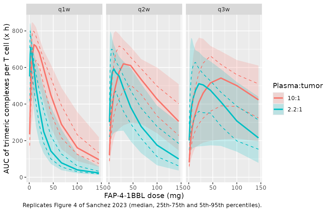
opt <- sum1 |>
  group_by(scenario, schedule) |>
  slice_max(med, n = 1, with_ties = FALSE) |>
  ungroup() |>
  select(scenario, schedule, sim_opt = dose) |>
  left_join(
    tribble(
      ~scenario, ~schedule, ~paper_opt, ~paper_lo, ~paper_hi,
      "2.2:1", "q1w", 3, 2, 10,
      "2.2:1", "q2w", 10, 4, 31,
      "2.2:1", "q3w", 21, 7, 65,
      "10:1", "q1w", 11, 5, 31,
      "10:1", "q2w", 33, 14, 80,
      "10:1", "q3w", 67, 23, 145
    ),
    by = c("scenario", "schedule")
  )
opt |>
  dplyr::rename("Plasma:tumor" = scenario, "Schedule" = schedule,
                "Simulated optimum (mg)" = sim_opt, "Figure 4 optimum (mg)" = paper_opt,
                "Figure 4 range low (mg)" = paper_lo, "Figure 4 range high (mg)" = paper_hi) |>
knitr::kable()| Plasma:tumor | Schedule | Simulated optimum (mg) | Figure 4 optimum (mg) | Figure 4 range low (mg) | Figure 4 range high (mg) |
|---|---|---|---|---|---|
| 10:1 | q1w | 10 | 11 | 5 | 31 |
| 10:1 | q2w | 30 | 33 | 14 | 80 |
| 10:1 | q3w | 67 | 67 | 23 | 145 |
| 2.2:1 | q1w | 3 | 3 | 2 | 10 |
| 2.2:1 | q2w | 10 | 10 | 4 | 31 |
| 2.2:1 | q3w | 21 | 21 | 7 | 65 |
# The median dose-response is flat near its peak, so the simulated optimum is
# checked against the paper's within-20%-of-maximum dose range rather than
# against the single optimum dose.
stopifnot(all(opt$sim_opt >= opt$paper_lo & opt$sim_opt <= opt$paper_hi))
The optimum doses agree with Figure 4. The simulated AUC is several-fold higher than the Figure 4 axis (largest median here 725 versus about 100 in the paper); see Assumptions and deviations.
Simulation 2: tumor FAP expression and the expected benefit
Typical-value simulation over the first 120 h: cibisatamab 100 mg over 2 h, then FAP-4-1BBL over 2 h at the 2.75 mg dose that maximizes trimeric complex formation in this window, or at a dose 100-fold higher. FAP expression varies over a grid of FAP-positive fibroblast percentages at the median 12,000 FAP/fibroblast.
grid2 <- tidyr::expand_grid(
  dose = c(2.75, 275),
  fap_pos_pct = c(1, 2, 5, 10, 15, 25, 40, 60, 80, 100)
) |>
  mutate(id = row_number())
ev2 <- bind_rows(
  grid2 |> transmute(id, time = 0, amt = 100, rate = 50, evid = 1, cmt = "central_cibisatamab"),
  grid2 |> transmute(id, time = 2, amt = dose, rate = dose / 2, evid = 1, cmt = "central"),
  grid2 |> transmute(id, time = 120, amt = 0, rate = 0, evid = 0, cmt = "central")
) |>
  arrange(id, time, desc(evid))
sim2 <- rxSolve(rxode2::zeroRe(ui_combo), ev2, params = grid2 |> select(id, fap_pos_pct),
                returnType = "data.frame") |>
  select(id, trimer_avg, fold_kill, kill_abs) |>
  left_join(grid2, by = "id")
#> Warning: No sigma parameters in the model
#> ℹ omega/sigma items treated as zero: 'etalvc', 'etalcl', 'etalvp', 'etalvmax', 'etalkm'

sim2 |>
  select(dose, fap_pos_pct, trimer_avg, fold_kill, kill_abs) |>
  pivot_longer(c(trimer_avg, fold_kill, kill_abs)) |>
  mutate(name = factor(name, c("trimer_avg", "fold_kill", "kill_abs"),
                       c("Average trimers per T cell", "Fold increase vs monotherapy",
                         "Killing vs monotherapy without FAP+"))) |>
  ggplot(aes(fap_pos_pct, value, colour = factor(dose))) +
  geom_line() + geom_point() +
  facet_wrap(~name, scales = "free_y") +
  labs(x = "FAP-positive fibroblasts in tumor (%)", y = NULL, colour = "Dose (mg)",
       caption = "Typical-value counterpart of Figure 5 of Sanchez 2023.")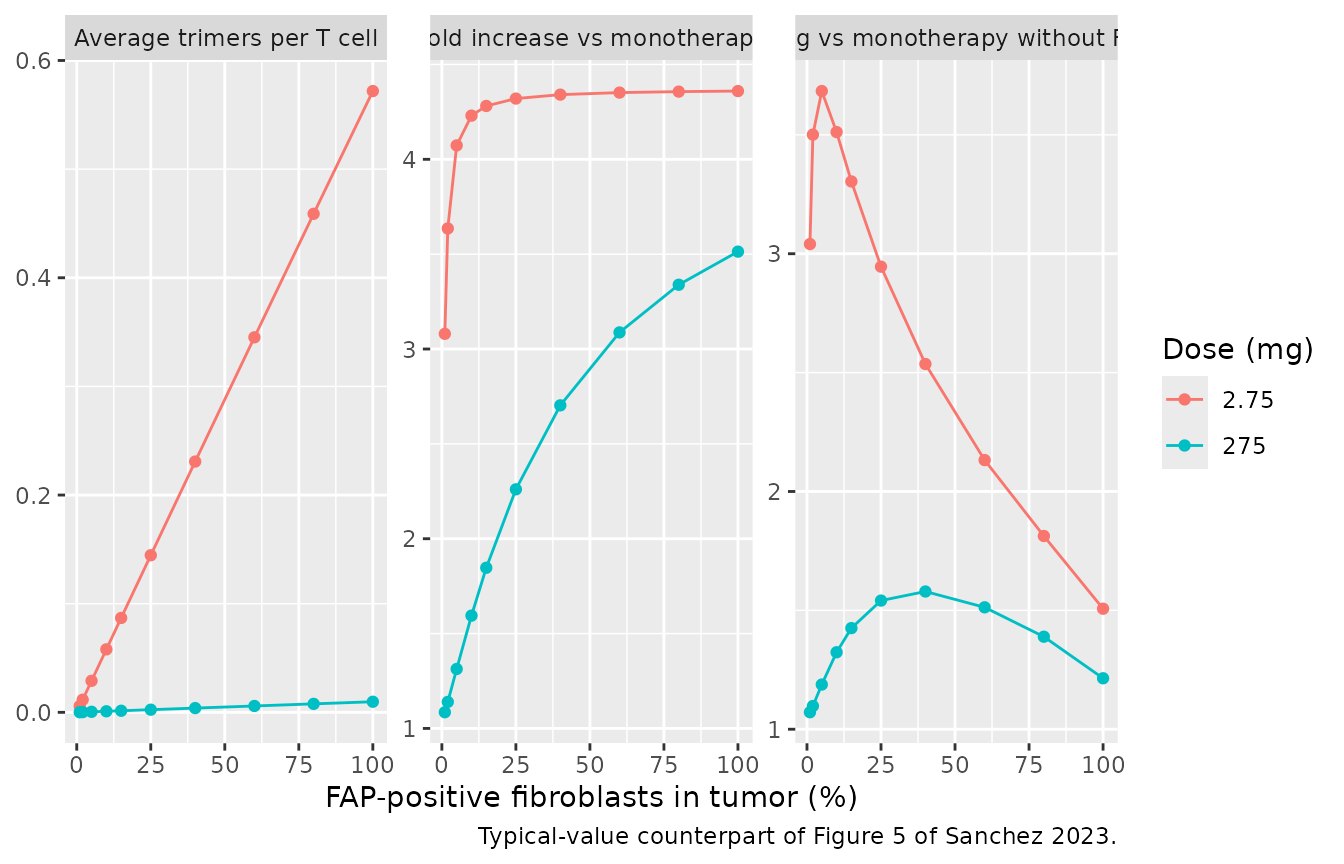
hi <- sim2 |> filter(dose == 2.75)
stopifnot(
  # Figure 5: at the trimer-maximizing dose the fold increase is near its
  # maximum once a few percent of the fibroblasts express FAP ...
  all(hi$fold_kill[hi$fap_pos_pct >= 10] > 4),
  # ... while absolute killing falls with more FAP-positive fibroblasts.
  hi$kill_abs[hi$fap_pos_pct == 100] < hi$kill_abs[hi$fap_pos_pct == 10],
  # A 100-fold higher dose forms far fewer trimers.
  all(sim2$trimer_avg[sim2$dose == 275] < hi$trimer_avg)
)
Simulation 3 (Figure 6) layers permutation tests over Simulation 2-type virtual patients to size dose-ranging cohorts; it is a statistical design exercise over the same model and is not reproduced here.
FAP-4-1BBL plasma PK (PKNCA)
The paper reports no NCA; the block below documents the single-dose typical exposure implied by the Table S1 parameters for three doses near the Simulation 1 optima.
ev_pk <- tibble(dose_mg = c(3, 10, 21), id = 1:3)
ev_pk <- bind_rows(
  ev_pk |> transmute(id, dose_mg, time = 0, amt = dose_mg, rate = dose_mg / 2, evid = 1, cmt = "central"),
  ev_pk |> tidyr::crossing(time = c(0, 1, 2, 3, 4, 6, 8, 12, 24, 48, 72, 96, 168, 336, 504)) |>
    transmute(id, dose_mg, time, amt = 0, rate = 0, evid = 0, cmt = "central")
) |>
  arrange(id, time, desc(evid))
sim_pk <- rxSolve(rxode2::zeroRe(ui_dose), ev_pk, returnType = "data.frame")
#> Warning: No sigma parameters in the model
#> ℹ omega/sigma items treated as zero: 'etalvc', 'etalcl', 'etalvp', 'etalvmax', 'etalkm'
conc <- sim_pk |>
  filter(!is.na(Cc)) |>
  select(id, time, Cc) |>
  left_join(distinct(ev_pk, id, dose_mg), by = "id")
dose_df <- ev_pk |> filter(evid == 1) |> select(id, dose_mg, time, amt)
o_conc <- PKNCAconc(conc, Cc ~ time | dose_mg + id)
o_dose <- PKNCAdose(dose_df, amt ~ time | dose_mg + id, route = "intravascular", duration = 2)
o_data <- PKNCAdata(o_conc, o_dose,
                    intervals = data.frame(start = 0, end = Inf, cmax = TRUE, tmax = TRUE,
                                           aucinf.obs = TRUE, half.life = TRUE))
nca <- pk.nca(o_data)
as.data.frame(nca$result) |>
  filter(PPTESTCD %in% c("cmax", "tmax", "aucinf.obs", "half.life")) |>
  select(dose_mg, PPTESTCD, PPORRES) |>
  pivot_wider(names_from = PPTESTCD, values_from = PPORRES) |>
  dplyr::rename("Dose (mg)" = dose_mg, "Cmax (mg/L)" = cmax, "Tmax (h)" = tmax,
                "AUC0-inf (mg*h/L)" = aucinf.obs, "t1/2 (h)" = half.life) |>
knitr::kable(digits = 3)| Dose (mg) | Cmax (mg/L) | Tmax (h) | t1/2 (h) | AUC0-inf (mg*h/L) |
|---|---|---|---|---|
| 3 | 0.772 | 2 | 40.703 | 30.840 |
| 10 | 2.581 | 2 | 40.638 | 114.830 |
| 21 | 5.440 | 2 | 40.528 | 277.284 |
Assumptions and deviations
-
Vmax units. Table S1 prints Vmax as 0.455 ug/h, but
the deposited dose-selection code subtracts
Vmax * C / (C + Km)from an amount in mg with concentrations in mg/L, so Vmax is 0.455 mg/h. Only the mg/h reading puts the Simulation 1 optimum doses where Figure 4 has them (with 0.455 ug/h the nonlinear clearance is negligible and every optimum moves several-fold lower). The volumes and clearances are in mL and mL/h in the code (Table S1 labels V1 and V2 in L); they are packaged as 3.77 L, 0.83 L, 0.0154 L/h and 0.0219 L/h. -
Signal under FAP-4-1BBL costimulation. The
deposited clinical code multiplies the monotherapy Signal by an added
value, capped at SignalMAX. The in vitro model sets that multiplier to
Signal2 divided by the monotherapy Signal at 20 nM cibisatamab (1.39,
the “39% increase in Signal” of the Supplementary Materials and Methods)
whenever FAP-4-1BBL is in the well, which reproduces Equation 3 at the
tested condition and the Figure 3c contour. The clinical combination
model keeps the code default
added_value = 1; the paper describes the clinical increase only as proportional to the trimeric complex formation, without a usable form. -
4-1BB binding form. Equation 16 degrades only the
free 4-1BB, but the deposited code lets the total 4-1BB pool follow the
per-cell turnover of Model 1 and redistributes it by binding. The
packaged models use the code form: it puts the in vitro trimer maximum
at 0.37 nM as Figure 3c does, while the Equation 16 form moves it to
about 1 nM. Equation 17 also prints
koff_FAP x FAP-4-1BBLwhere the code (and mass balance) haskoff_FAP x Trimeric; the code form is used. - Stop time in the clinic. Signal and basal 4-1BB synthesis switch off 16.2 h after the first cibisatamab dose, so the cibisatamab combination model is meaningful over the 120-h and one-week windows of Simulations 2 and 3, not for multi-cycle regimens. Simulation 1 uses the separate constant-4-1BB model. In the in vitro model basal synthesis continues in cibisatamab-free wells, as the deposited Monolix code specifies.
-
T-cell count. The deposited dose-selection code
initializes 4-1BB from
E_T_ratio / 100T cells per tumor cell but normalizes trimers byE_T_ratio x 40% x 0.4; both packaged clinical models use the latter throughout. The 4-1BB concentration is about 1e-5 nM either way, far below the FAP and drug concentrations, so the choice does not move the results. The in vitro model applies the same 40% x 0.4 T-cell factors to the PBMC count, which the paper does not state for the wells; the receptor concentration is again negligible against FAP and drug. - Clinical FAP expression. Simulation 1 fixes FAP at 12% FAP-positive fibroblasts and 12,000 FAP/fibroblast as stated in the Supplementary Materials and Methods. The deposited code takes these medians from an H-score script that is not part of the supplement. With the stated medians the simulated trimeric-complex AUC is about seven-fold above the Figure 4 axis; trimer formation is linear in FAP at these receptor levels, so the optimum doses are unaffected while the absolute AUC is. Simulation 2 here uses a deterministic FAP grid instead of the H-score sampling.
- Cibisatamab tumor distribution. Table S1 lists the same 0.06 and 0.137 1/h rate constants for cibisatamab (labelled a 2.5:1 ratio) as for FAP-4-1BBL; the deposited code shares them between the two drugs.
- Model 1 parameter values. Table 2 and Table S1 are used. The parameter block of the deposited Monolix project holds slightly different values (for example EC50 13.6 nM, residual SD 7.25), which are the starting values of a later run rather than the reported estimates.
- Observed Model 1 values in the first figure were read by eye off Figure S4; Figure 3a means likewise. They are qualitative comparators.