Donepezil oral and transdermal patch (Jung 2022)
Source:vignettes/articles/Jung_2022_donepezil.Rmd
Jung_2022_donepezil.RmdModel and source
- Citation: Jung W, Jung H, Vu N-AT, Kim G-Y, Kim G-W, Chae J-w, Kim T, Yun H-y. Model-Based Equivalent Dose Optimization to Develop New Donepezil Patch Formulation. Pharmaceutics. 2022;14(2):244. doi:10.3390/pharmaceutics14020244. Unrounded final estimates and the NONMEM control stream are published as Code S2 (‘case 1, base model’, OFV 1443.703) in the supplement of Jung W, Ryu H-j, Chae J-w, Yun H-y. Fractal Kinetic Implementation in Population Pharmacokinetic Modeling. Pharmaceutics. 2023;15(1):304. doi:10.3390/pharmaceutics15010304.
- Description: Two-compartment population PK model for donepezil given orally or as a once-weekly transdermal patch in healthy adult Korean men (Jung 2022). Oral dose enters a gut depot absorbed at first-order Ka; patch dose enters a formulation reservoir that empties at first-order Kt through two transit compartments (same Kt) into the same central compartment. Both routes share one central and one peripheral compartment and one linear clearance. The fraction of the nominal patch strength that reaches the skin is fixed from the in-vitro dissolution equation (Jung 2022 Eq. 3) at the one-week (168 h) wear time used throughout the study and its simulations.
- Article: https://doi.org/10.3390/pharmaceutics14020244
- Control stream with unrounded estimates (Code S2 of a later paper by the same group): https://doi.org/10.3390/pharmaceutics15010304
Jung 2022 built one integrated population PK model for a once-daily
10 mg oral donepezil tablet and a once-weekly donepezil transdermal
patch, then used it to find the patch strengths whose simulated
steady-state AUC and Cmax are bioequivalent to the tablet. The two
routes share one central compartment, one peripheral compartment and one
clearance. Oral drug is absorbed from a gut depot at first-order
Ka; patch drug leaves a skin reservoir at first-order
Kt and passes through two transit compartments with the
same Kt before reaching plasma (Jung 2022 Eqs. 1, 2 and 4,
Figure 1).
The amount that enters the skin reservoir is not the nominal patch strength. Jung 2022 Eq. 3 fits the in-vitro dissolution profile as
with D the wear time in hours, and scales it by 0.74,
the ratio of the drug released in the clinical study (measured from the
residue left in used patches) to the in-vitro release. At the one-week
wear used in the study and in every simulation of the paper this gives
0.74 * 0.78257 * 168 / (168 + 8.481) = 0.5513, carried in
the model as the fixed bioavailability f(depot_td). Dose
the nominal patch strength.
The same authors refit this model unchanged as the “base model” of
Case 1 in a 2023 methods paper on fractal absorption kinetics, and
published its NONMEM control stream (Code S2) there. Code S2 reproduces
Jung 2022 Table 3 exactly (identical OFV 1443.703, every estimate
rounding to the Table 3 value), so the unrounded Code S2 values are used
here. The fractal refit of the same data ships separately as
Jung_2023_donepezil_singledose.
Population
Twelve healthy male volunteers aged 18-45 years were enrolled in a randomised, open-label, two-treatment, two-sequence, two-period crossover study (TL/WZ/19/001141). Nine completed both periods and form the analysis set (Jung 2022 Section 3.1, Table 1): age 24-33 years (median 30.0), weight 55.7-80.9 kg (median 63.1), BMI 19.8-27.3 kg/m^2, all male and all Asian. The test period was one 108 mg / 96 cm^2 patch worn on the torso or back for one week; the reference period was 10 mg Aricept once daily for seven days, with a washout of at least 21 days. Blood was sampled to 312 h. The model has no covariates.
readModelDb("Jung_2022_donepezil")()$population |> str()
#> List of 14
#>  $ species       : chr "human"
#>  $ n_subjects    : num 9
#>  $ n_studies     : num 1
#>  $ age_range     : chr "24-33 years"
#>  $ age_median    : chr "30.0 years"
#>  $ weight_range  : chr "55.7-80.9 kg"
#>  $ weight_median : chr "63.1 kg"
#>  $ sex_female_pct: num 0
#>  $ race_ethnicity: Named num 100
#>   ..- attr(*, "names")= chr "Asian"
#>  $ disease_state : chr "Healthy adult male volunteers"
#>  $ dose_range    : chr "Donepezil 10 mg oral tablet (Aricept) once daily for 7 days, or one 108 mg / 96 cm2 transdermal patch worn for "| __truncated__
#>  $ regions       : chr "Not stated; ethics approval by Raptim Research Ltd (Mumbai, India), sponsor and analysts in the Republic of Korea"
#>  $ n_observations: num 383
#>  $ notes         : chr "Randomised, open-label, two-treatment, two-sequence, two-period crossover bioequivalence study (TL/WZ/19/001141"| __truncated__
Source trace
| Equation / parameter | Value | Source location |
|---|---|---|
d/dt(depot_oral) = -ka * depot_oral |
n/a | Jung 2022 Eq. 1; Code S2 $DES DADT(1) |
d/dt(depot_td), d/dt(transit1),
d/dt(transit2) (one Kt) |
n/a | Jung 2022 Eq. 2; Code S2 $DES DADT(4)-DADT(6) |
d/dt(central), d/dt(peripheral1),
kel = CL/Vc, kcp = Q/Vc,
kpc = Q/Vp
|
n/a | Jung 2022 Eq. 4; Code S2 $PK / $DES
|
f(depot_td) = 0.74 * 0.78257 * 168 / (168 + 8.481) |
0.5513 | Jung 2022 Eq. 3 with the one-week wear of Section 2.1 |
Cc = 1000 * central / vc (ng/mL) |
n/a | Code S2 $ERROR,
IPRED = A(2)/(VC/1000)
|
lka |
log(0.0496711) 1/h | Table 3 Ka 0.0497; Code S2 THETA(1) |
lcl |
log(10.0268) L/h | Table 3 CL 10; Code S2 THETA(2) |
lvc |
log(26.2189) L | Table 3 Vc 26.2; Code S2 THETA(3) |
lvp |
log(562.037) L | Table 3 Vp 562; Code S2 THETA(4) |
lq |
log(15.6292) L/h | Table 3 Q 15.6; Code S2 THETA(5) |
lktr |
log(0.0270191) 1/h | Table 3 Kt 0.027; Code S2 THETA(6) |
etalka |
0.00968106 (9.9% CV) | Table 3; Code S2 OMEGA(1) |
etalcl |
0.130076 (37.3% CV) | Table 3; Code S2 OMEGA(2) |
etalvc |
0.197923 (46.8% CV) | Table 3; Code S2 OMEGA(3) |
etalktr |
0.020045 (14.2% CV) | Table 3; Code S2 OMEGA(4) |
addSd |
2.89074 ng/mL | Table 3 additive error 2.89; Code S2 THETA(7) |
propSd |
0.0795173 | Table 3 proportional error 0.0795; Code S2 THETA(8) |
The Table 3 “IIV” column is a variance:
sqrt(exp(omega) - 1) recovers its printed CV% for every row
(for example sqrt(exp(0.13) - 1) = 37.3%).
mod <- readModelDb("Jung_2022_donepezil")
ui <- rxode2::rxode2(mod)
#> ℹ parameter labels from comments will be replaced by 'label()'
omega_cv <- 100 * sqrt(exp(diag(ui$omega)) - 1)
published_cv <- c(etalka = 9.9, etalcl = 37.3, etalvc = 46.8, etalktr = 14.2)
round(rbind(model = omega_cv[names(published_cv)], published = published_cv), 1)
#>           etalka etalcl etalvc etalktr
#> model        9.9   37.3   46.8    14.2
#> published    9.9   37.3   46.8    14.2
stopifnot(max(abs(omega_cv[names(published_cv)] - published_cv)) < 0.1)
Structural checks on the typical subject
Both routes are linear, so the total exposure of the typical subject
is fixed by clearance alone: AUC(0,inf) = F * Dose / CL.
The oral arm (seven 10 mg doses, F = 1) and the patch arm
(108 mg, F = 0.5513) are integrated with tight tolerances
on a grid long enough for the 562 L peripheral volume to empty.
typ <- rxode2::zeroRe(mod)
#> ℹ parameter labels from comments will be replaced by 'label()'
f_td <- exp(ui$theta[["lfdepot_td"]])
cl_typ <- exp(ui$theta[["lcl"]])
grid <- sort(unique(c(seq(0, 200, by = 0.1), seq(200, 4000, by = 1))))

ev_oral_typ <- rxode2::et(amt = 10, cmt = "depot_oral", time = 0, ii = 24, addl = 6) |>
  rxode2::et(grid, cmt = "central")
ev_patch_typ <- rxode2::et(amt = 108, cmt = "depot_td", time = 0) |>
  rxode2::et(grid, cmt = "central")

trap <- function(t, y) sum(diff(t) * (head(y, -1) + tail(y, -1)) / 2)
solve_typ <- function(ev) {
  as.data.frame(rxode2::rxSolve(typ, ev, rtol = 1e-10, atol = 1e-12, maxsteps = 1e6))
}
s_oral_typ <- solve_typ(ev_oral_typ)
#> ℹ omega/sigma items treated as zero: 'etalka', 'etalcl', 'etalvc', 'etalktr'
s_patch_typ <- solve_typ(ev_patch_typ)
#> ℹ omega/sigma items treated as zero: 'etalka', 'etalcl', 'etalvc', 'etalktr'

identity <- tibble::tibble(
  arm = c("Oral 10 mg x 7", "Patch 108 mg"),
  expected = c(70 / cl_typ, f_td * 108 / cl_typ) * 1000,
  simulated = c(trap(s_oral_typ$time, s_oral_typ$Cc), trap(s_patch_typ$time, s_patch_typ$Cc))
) |>
  mutate(pct_diff = 100 * (simulated - expected) / expected)
knitr::kable(identity, digits = c(0, 1, 1, 4),
caption = "Typical-subject AUC(0,inf) (ng*h/mL) against F * Dose / CL.")| arm | expected | simulated | pct_diff |
|---|---|---|---|
| Oral 10 mg x 7 | 6981.3 | 6981.2 | -0.0013 |
| Patch 108 mg | 5937.8 | 5937.8 | 0.0002 |
# Deterministic solve against its own closed form; the residual (measured
# ~0.001%) is the trapezoid on the grid plus the concentration left at 4000 h.
# Dropping the Eq. 3 fraction or a digit of CL moves it by tens of percent.
stopifnot(max(abs(identity$pct_diff)) < 0.02)
The patch identity is also an independent check of Eq. 3. The typical patch AUC is 5938 ngh/mL; the observed mean AUCinf of the nine patch subjects is 5909 ngh/mL (Jung 2022 Table 2). Dosing the nominal 108 mg without the Eq. 3 fraction would predict about 10 800 ng*h/mL, so the delivered fraction is a load-bearing part of the model, not a detail.
Virtual cohort and simulation
The study cohort is reproduced as two arms of 200 virtual subjects each (the model has no covariates, so the arms differ only in their random effects): the reference regimen of 10 mg once daily for seven days and the test regimen of a single 108 mg patch, both observed to 312 h as in the study.
rxode2::rxSetSeed(20220120)
n_arm <- 200
obs_times <- sort(unique(c(seq(0, 24, by = 0.5), seq(25, 312, by = 1))))

make_arm <- function(n, treatment, id_offset, dose_rows) {
  ids <- id_offset + seq_len(n)
  doses <- tidyr::crossing(id = ids, dose_rows) |>
    mutate(evid = 1L)
  obs <- tidyr::crossing(id = ids, time = obs_times) |>
    mutate(amt = 0, cmt = "central", evid = 0L)
  bind_rows(doses, obs) |>
    mutate(treatment = treatment) |>
    arrange(id, time, desc(evid))
}

events <- bind_rows(
  make_arm(n_arm, "Oral", 0L,
           tibble::tibble(time = 24 * (0:6), amt = 10, cmt = "depot_oral")),
  make_arm(n_arm, "Patch", n_arm,
           tibble::tibble(time = 0, amt = 108, cmt = "depot_td"))
)
stopifnot(!anyDuplicated(unique(events[, c("id", "time", "evid")])))

sim <- rxode2::rxSolve(mod, events = events, keep = "treatment", maxsteps = 1e6) |>
  as.data.frame()
#> ℹ parameter labels from comments will be replaced by 'label()'
stopifnot(!anyNA(sim$Cc))
Replicate published figures
# Replicates Figure 2 of Jung 2022: VPC of donepezil after oral (upper) and
# transdermal patch (lower) administration.
sim |>
  group_by(treatment, time) |>
  summarise(
    Q05 = quantile(Cc, 0.05),
    Q50 = quantile(Cc, 0.50),
    Q95 = quantile(Cc, 0.95),
    .groups = "drop"
  ) |>
  ggplot(aes(time, Q50)) +
  geom_ribbon(aes(ymin = Q05, ymax = Q95), alpha = 0.25) +
  geom_line() +
  facet_wrap(~treatment, ncol = 1, scales = "free_y") +
  labs(x = "Time (h)", y = "Donepezil (ng/mL)",
       title = "Simulated 5th, 50th and 95th percentiles",
       caption = "Replicates Figure 2 of Jung 2022 (200 virtual subjects per arm).") +
  theme_bw()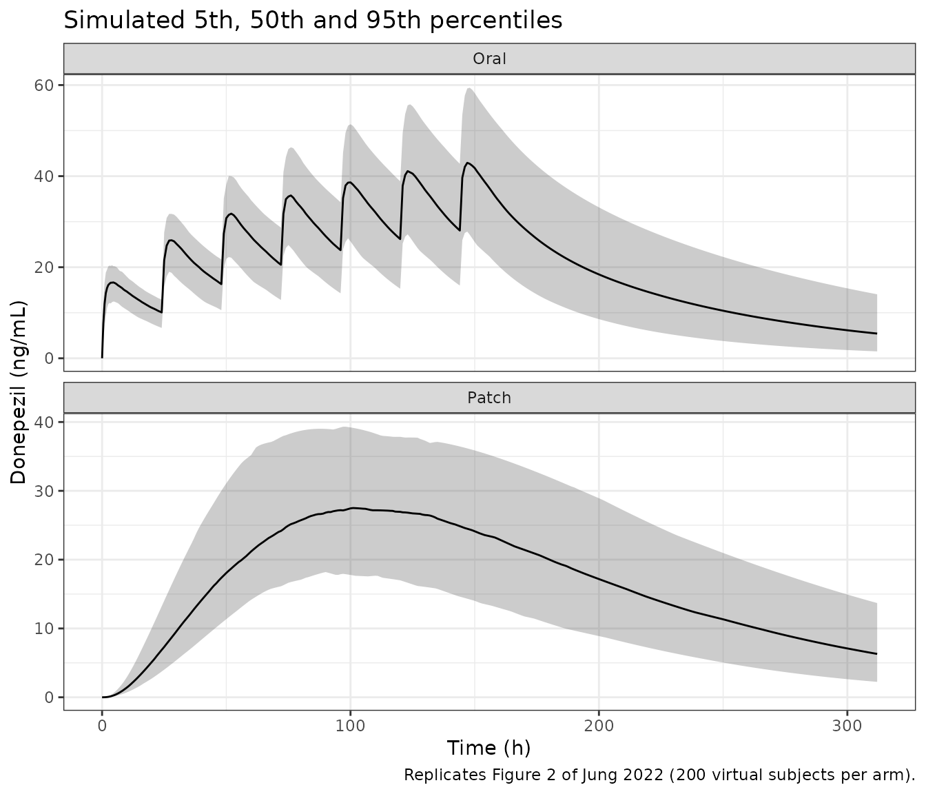
PKNCA validation
Jung 2022 Table 2 reports arithmetic means for three analyses: the first oral dose (0-24 h), the full oral course (0-312 h) and the patch (0-312 h). The oral profile is entered twice, once truncated at 24 h with only the first dose, so that each analysis is its own PKNCA group.
conc_all <- sim |>
  filter(!is.na(Cc)) |>
  select(id, time, Cc, treatment)

conc_nca <- bind_rows(
  conc_all |> filter(treatment == "Oral", time <= 24) |> mutate(analysis = "Oral (0-24 h)"),
  conc_all |> filter(treatment == "Oral") |> mutate(analysis = "Oral (0-312 h)"),
  conc_all |> filter(treatment == "Patch") |> mutate(analysis = "Patch (0-312 h)")
)
# Time-zero anchor for every subject (pre-dose Cc = 0 for extravascular dosing).
conc_nca <- bind_rows(
  conc_nca,
  conc_nca |> distinct(id, analysis) |> mutate(time = 0, Cc = 0)
) |>
  distinct(id, analysis, time, .keep_all = TRUE) |>
  arrange(analysis, id, time)

dose_all <- events |>
  filter(evid == 1) |>
  select(id, time, amt, treatment)
dose_nca <- bind_rows(
  dose_all |> filter(treatment == "Oral", time == 0) |> mutate(analysis = "Oral (0-24 h)"),
  dose_all |> filter(treatment == "Oral") |> mutate(analysis = "Oral (0-312 h)"),
  dose_all |> filter(treatment == "Patch") |> mutate(analysis = "Patch (0-312 h)")
)

conc_obj <- PKNCA::PKNCAconc(conc_nca, Cc ~ time | analysis + id)
dose_obj <- PKNCA::PKNCAdose(dose_nca, amt ~ time | analysis + id)

intervals <- bind_rows(
  data.frame(analysis = "Oral (0-24 h)", start = 0, end = 24,
             cmax = TRUE, tmax = TRUE, auclast = TRUE, aucinf.obs = FALSE, half.life = FALSE),
  data.frame(analysis = c("Oral (0-312 h)", "Patch (0-312 h)"), start = 0, end = Inf,
             cmax = TRUE, tmax = TRUE, auclast = TRUE, aucinf.obs = TRUE, half.life = TRUE)
)

nca_res <- PKNCA::pk.nca(PKNCA::PKNCAdata(conc_obj, dose_obj, intervals = intervals))
Comparison against published NCA
Jung 2022 Table 2 reports means, so the simulated results are
summarised as arithmetic means before comparison. AUCinf of
the first oral dose (575 ng*h/mL in the paper) is extrapolated from 24 h
of data with a 22 h half-life estimated within that window and is not
compared.
sim_mean <- as.data.frame(nca_res$result) |>
  filter(PPTESTCD %in% c("cmax", "tmax", "auclast", "aucinf.obs", "half.life")) |>
  group_by(analysis, PPTESTCD) |>
  summarise(value = mean(PPORRES, na.rm = TRUE), .groups = "drop") |>
  tidyr::pivot_wider(names_from = PPTESTCD, values_from = value)

published <- tibble::tribble(
  ~analysis,         ~cmax, ~tmax,  ~auclast, ~aucinf.obs, ~half.life,
  "Oral (0-24 h)",   20.26,   3.11,   286.62,          NA,        NA,
  "Oral (0-312 h)",  53.86, 146.33,  6111.08,     6873.40,     37.74,
  "Patch (0-312 h)", 28.62, 106.67,  5285.59,     5909.34,     71.17
)

cmp <- nlmixr2lib::ncaComparisonTable(
  simulated = sim_mean,
  reference = published,
  by = "analysis",
  units = c(cmax = "ng/mL", tmax = "h", auclast = "ng*h/mL",
            aucinf.obs = "ng*h/mL", half.life = "h"),
  tolerance_pct = 20
)
knitr::kable(cmp, caption = "Simulated (mean of 200 per arm) vs. published (mean of 9) NCA. * differs from reference by >20%.")| NCA parameter | analysis | Reference | Simulated | % diff |
|---|---|---|---|---|
| Cmax (ng/mL) | Oral (0-24 h) | 20.3 | 16.9 | -16.6% |
| Cmax (ng/mL) | Oral (0-312 h) | 53.9 | 43.5 | -19.2% |
| Cmax (ng/mL) | Patch (0-312 h) | 28.6 | 28.8 | +0.5% |
| Tmax (h) | Oral (0-24 h) | 3.11 | 3.68 | +18.2% |
| Tmax (h) | Oral (0-312 h) | 146 | 147 | +0.5% |
| Tmax (h) | Patch (0-312 h) | 107 | 104 | -2.2% |
| AUC0-∞ (obs) (ng*h/mL) | Oral (0-24 h) | — | — | — |
| AUC0-∞ (obs) (ng*h/mL) | Oral (0-312 h) | 6870 | 7340 | +6.9% |
| AUC0-∞ (obs) (ng*h/mL) | Patch (0-312 h) | 5910 | 6270 | +6.2% |
| AUClast (ng*h/mL) | Oral (0-24 h) | 287 | 313 | +9.4% |
| AUClast (ng*h/mL) | Oral (0-312 h) | 6110 | 6660 | +9.0% |
| AUClast (ng*h/mL) | Patch (0-312 h) | 5290 | 5410 | +2.3% |
| t½ (h) | Oral (0-24 h) | — | — | — |
| t½ (h) | Oral (0-312 h) | 37.7 | 65.8 | +74.4%* |
| t½ (h) | Patch (0-312 h) | 71.2 | 74.6 | +4.8% |
num <- function(analysis, code) {
  v <- sim_mean[[code]][sim_mean$analysis == analysis]
  if (length(v) != 1L) stop("no unique row for ", analysis, " / ", code)
  v
}
pub <- function(analysis, code) {
  v <- published[[code]][published$analysis == analysis]
  if (length(v) != 1L) stop("no unique row for ", analysis, " / ", code)
  v
}
pct <- function(analysis, code) 100 * (num(analysis, code) / pub(analysis, code) - 1)

# Exposure gates on the centre of a 200-subject cohort. The CV of individual
# AUC is ~37% (the IIV on CL), so the standard error of a 200-subject mean is
# ~3%; the 15% bound sits > 4 SE out and still catches a mis-transcribed CL,
# a missing Eq. 3 fraction (+80%) or a wrong unit.
stopifnot(
  abs(pct("Oral (0-312 h)", "aucinf.obs")) < 15,
  abs(pct("Patch (0-312 h)", "aucinf.obs")) < 15,
  abs(pct("Patch (0-312 h)", "cmax")) < 20,
  # Patch Tmax is set by the three-step Kt chain (mean transit 3 / Kt = 111 h).
  abs(pct("Patch (0-312 h)", "tmax")) < 20
)
The patch arm agrees with Table 2 on every row, and the AUCs of both
routes agree to within 10%. The simulated mean AUCs sit about 6-7% above
the typical values of the identity check above, which is the expected
gap between the mean and the median of a log-normal exposure:
exp(0.130 / 2) = 1.067 for the IIV on CL. Two rows differ
more:
-
Oral Cmax is 15-20% below the observed means, both
after the first dose and at the end of the course, while the oral Tmax
and AUC agree. The estimated
Ka(0.0497 1/h) is slow for an immediate-release tablet; the authors note estimation difficulties from flip-flop kinetics, and a slow absorption constant flattens the oral peak more than it shifts its timing. The model is shipped as estimated. - Oral half-life (starred). The oral course ends at 144 h, so the 0-312 h window holds only 168 h of washout, over which the 562 L peripheral compartment is still returning drug. The published 37.7 h (and 22.3 h from the first 24 h alone) are distribution-phase slopes from sparse sampling; the simulated value comes from a denser grid whose last points lie further into the terminal phase. The patch half-life, fitted after a longer absorption tail, agrees.
Equivalent patch dose (Table 4 and Figure 3)
Jung 2022 simulated 10 mg oral donepezil once daily against once-weekly patches and compared AUC and Cmax over the steady-state week 672-840 h. The typical-subject ratios are deterministic, and reproduce the published point estimates (which come from a 100-per-arm stochastic simulation):
ss_grid <- seq(672, 840, by = 0.25)
ss_solve <- function(ev) {
  s <- as.data.frame(rxode2::rxSolve(typ, ev, rtol = 1e-10, atol = 1e-12, maxsteps = 1e6))
  s[s$time >= 672 & s$time <= 840, ]
}
ref_ss <- ss_solve(rxode2::et(amt = 10, cmt = "depot_oral", time = 0, ii = 24, addl = 34) |>
                     rxode2::et(ss_grid, cmt = "central"))
#> ℹ omega/sigma items treated as zero: 'etalka', 'etalcl', 'etalvc', 'etalktr'
patch_ratio <- function(dose) {
  s <- ss_solve(rxode2::et(amt = dose, cmt = "depot_td", time = 0, ii = 168, addl = 4) |>
                  rxode2::et(ss_grid, cmt = "central"))
  c(auc = 100 * trap(s$time, s$Cc) / trap(ref_ss$time, ref_ss$Cc),
    cmax = 100 * max(s$Cc) / max(ref_ss$Cc))
}
r114 <- patch_ratio(114)
#> ℹ omega/sigma items treated as zero: 'etalka', 'etalcl', 'etalvc', 'etalktr'
r146 <- patch_ratio(146)
#> ℹ omega/sigma items treated as zero: 'etalka', 'etalcl', 'etalvc', 'etalktr'

tab4 <- tibble::tibble(
  patch = c("114 mg / 101.3 cm2", "114 mg / 101.3 cm2", "146 mg / 129.8 cm2", "146 mg / 129.8 cm2"),
  metric = c("AUC", "Cmax", "AUC", "Cmax"),
  published_ratio = c(91.16, 86.66, 115.63, 108.77),
  published_ci90 = c("85.61-97.06", "82.07-91.51", "108.62-123.09", "102.98-114.88"),
  typical_ratio = c(r114[["auc"]], r114[["cmax"]], r146[["auc"]], r146[["cmax"]])
) |>
  mutate(pct_diff = 100 * (typical_ratio / published_ratio - 1))

tab4 |>
  dplyr::rename(
    "Patch" = patch, "Metric" = metric, "Published ratio (%)" = published_ratio,
    "Published 90% CI" = published_ci90, "Typical-subject ratio (%)" = typical_ratio,
    "% diff" = pct_diff
  ) |>
knitr::kable(digits = 2, caption = "Replicates Table 4 of Jung 2022 (test patch / reference 10 mg oral daily).")| Patch | Metric | Published ratio (%) | Published 90% CI | Typical-subject ratio (%) | % diff |
|---|---|---|---|---|---|
| 114 mg / 101.3 cm2 | AUC | 91.16 | 85.61-97.06 | 89.78 | -1.52 |
| 114 mg / 101.3 cm2 | Cmax | 86.66 | 82.07-91.51 | 88.63 | 2.28 |
| 146 mg / 129.8 cm2 | AUC | 115.63 | 108.62-123.09 | 114.98 | -0.56 |
| 146 mg / 129.8 cm2 | Cmax | 108.77 | 102.98-114.88 | 113.51 | 4.36 |
# Deterministic quantities. Every typical-subject ratio lies inside the published
# 90% CI; the AUC ratios are within 2% of the published point estimates. A
# mis-transcribed Kt, Eq. 3 constant or unit moves them by far more.
ci <- do.call(rbind, lapply(strsplit(tab4$published_ci90, "-"), as.numeric))
stopifnot(
  all(tab4$typical_ratio > ci[, 1] & tab4$typical_ratio < ci[, 2]),
  max(abs(tab4$pct_diff[tab4$metric == "AUC"])) < 2.5,
  max(abs(tab4$pct_diff)) < 6
)
# Replicates Figure 3 of Jung 2022: 10 mg oral daily vs 114 mg (upper) and
# 146 mg (lower) weekly patches, median and 5th-95th percentiles.
rxode2::rxSetSeed(20220121)
fig3_times <- seq(0, 840, by = 2)
make_fig3 <- function(n, id_offset, dose_rows, label) {
  ids <- id_offset + seq_len(n)
  bind_rows(
    tidyr::crossing(id = ids, dose_rows) |> mutate(evid = 1L),
    tidyr::crossing(id = ids, time = fig3_times) |> mutate(amt = 0, cmt = "central", evid = 0L)
  ) |>
    mutate(regimen = label) |>
    arrange(id, time, desc(evid))
}
ev_fig3 <- bind_rows(
  make_fig3(100, 0L, tibble::tibble(time = 24 * (0:34), amt = 10, cmt = "depot_oral"), "Oral 10 mg daily"),
  make_fig3(100, 100L, tibble::tibble(time = 168 * (0:4), amt = 114, cmt = "depot_td"), "Patch 114 mg weekly"),
  make_fig3(100, 200L, tibble::tibble(time = 168 * (0:4), amt = 146, cmt = "depot_td"), "Patch 146 mg weekly")
)
stopifnot(!anyDuplicated(unique(ev_fig3[, c("id", "time", "evid")])))
sim3 <- rxode2::rxSolve(mod, events = ev_fig3, keep = "regimen", maxsteps = 1e6) |>
  as.data.frame()

summ3 <- sim3 |>
  group_by(regimen, time) |>
  summarise(Q05 = quantile(Cc, 0.05), Q50 = quantile(Cc, 0.5), Q95 = quantile(Cc, 0.95),
            .groups = "drop")
oral3 <- filter(summ3, regimen == "Oral 10 mg daily")
bind_rows(
  bind_rows(oral3, filter(summ3, regimen == "Patch 114 mg weekly")) |> mutate(panel = "114 mg patch"),
  bind_rows(oral3, filter(summ3, regimen == "Patch 146 mg weekly")) |> mutate(panel = "146 mg patch")
) |>
  ggplot(aes(time, Q50, colour = regimen, fill = regimen)) +
  geom_ribbon(aes(ymin = Q05, ymax = Q95), alpha = 0.2, colour = NA) +
  geom_line() +
  facet_wrap(~panel, ncol = 1) +
  scale_colour_manual(values = c("grey40", "forestgreen", "firebrick")) +
  scale_fill_manual(values = c("grey40", "forestgreen", "firebrick")) +
  labs(x = "Time (h)", y = "Donepezil (ng/mL)", colour = NULL, fill = NULL,
       caption = "Replicates Figure 3 of Jung 2022 (100 virtual subjects per regimen).") +
  theme_bw() +
  theme(legend.position = "bottom")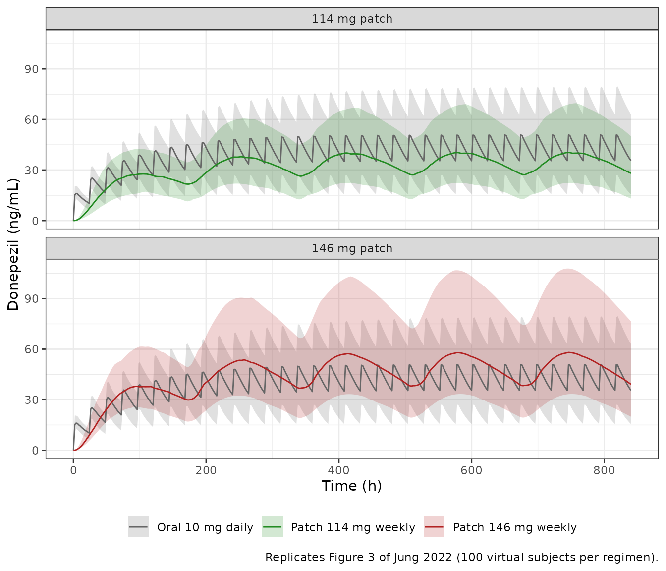
Assumptions and deviations
-
Unrounded estimates from the later control stream.
Jung 2022 Table 3 prints rounded estimates. Code S2 of Jung 2023 (the
same authors’ fractal kinetics paper) is the NONMEM control stream of
this model, fitted to the same data with the identical OFV 1443.703; its
$THETAand$OMEGAround to every Table 3 value and are used here. -
The patch delivered fraction is fixed at the one-week
wear. Eq. 3 is a function of wear time, and Code S2 applies it
to the patch dose amount in the dataset rather than inside the model.
Every patch in the study and in the paper’s simulations was worn for 168
h, so the model carries the resulting constant
F = 0.5513. For a different wear timeD(hours), override it withini(lfdepot_td = fixed(log(0.74 * 0.78257 * D / (D + 8.481)))). The in-vitro dissolution data behind Eq. 3 (supplementary Table S3) are not needed to use the model; the fitted constants are printed in Eq. 3. -
Patch removal is not modelled. The drug that has
entered the skin reservoir continues to transit to plasma after the
patch comes off, as in Eq. 2 and Code S2; the undelivered remainder is
excluded by
F. -
Typographical error in Eq. 4. The printed
central-compartment equation has the oral input as
KA * SKIN; Eq. 1 and Code S2 (KA*A(1)) both make itKA * GUT, which is what is implemented. - Bioequivalence simulation design. The paper describes a 2 x 2 crossover with 100 simulated subjects per group but not how the variability between periods was generated (the model has no inter-occasion variability). The Table 4 comparison therefore uses the deterministic typical-subject ratio, which should be close to the published geometric-mean ratio, and checks it against the published 90% confidence intervals rather than recomputing them.
- Study conduct. The sponsor and analysts were in the Republic of Korea; the ethics approval was issued by the institutional review board of Raptim Research (Mumbai, India). The paper does not state where subjects were dosed.
- No erratum or correction notice for Jung 2022 was found as of 2026-09-30.