Benzylpenicillin (Obura 2025)
Source:vignettes/articles/Obura_2025_benzylpenicillin.Rmd
Obura_2025_benzylpenicillin.RmdModel and source
- Citation: Obura B, Unsworth J, Jimenez-Valverde A, Waitt C, Das S, Hope W, Navaratnam K. Pharmacokinetics of Intrapartum Benzylpenicillin: Insights Into Candidate Regimens to Prevent Early Onset Neonatal Group B Streptococcus Disease. CPT Pharmacometrics Syst Pharmacol. 2025;14(9):1504-1514. doi:10.1002/psp4.70072. PMID: 40629558. PMCID: PMC12439288.
- Description: Two-compartment IV population PK model of intrapartum benzylpenicillin (penicillin G) in 12 labouring women at risk of early-onset neonatal Group B Streptococcus disease (Obura 2025), with a third, umbilical cord compartment linked to the maternal central compartment by first-order rate constants. Maternal plasma and umbilical cord blood concentrations are both observed. Pmetrics NPAG non-parametric fit; typical values are the weighted means of the joint density (Table 2) and inter-individual variability is a log-normal approximation built from the reported CV% and the CL-Vc correlation. No covariates were retained. Concentrations are total drug; the paper converts to unbound with a fixed 60% protein binding for target attainment.
- Article: https://doi.org/10.1002/psp4.70072
Obura 2025 characterises intrapartum benzylpenicillin (penicillin G) given to women at risk of having a baby with early-onset Group B Streptococcus (GBS) disease. A two-compartment maternal model is linked to an umbilical cord compartment, so that both maternal plasma and cord blood exposure can be simulated. The paper then uses Monte Carlo simulation to compare the standard UK regimen (3 g, then 1.5 g every 4 h) with lower and continuous-infusion alternatives, against an unbound-concentration target of 0.125 mg/L.
Population
Twelve pregnant women were enrolled at Liverpool Women’s Hospital, UK, between January 2022 and June 2023 (Obura 2025 Results, Table 1). Indications were preterm labour (n = 5), a GBS-positive antenatal swab (n = 4) and GBS bacteriuria (n = 3). Median (range) age was 30.5 (19-37) years and weight 75 (52-132) kg; BMI was 30.7 +/- 10.45 kg/m^2 and serum creatinine 0.56 +/- 0.12 mg/dL. Nine women were White and three Asian. All received a 3 g loading dose over about 30 min at the onset of labour, followed by 0 to 4 maintenance doses of 1.5 g every 4 h until delivery. The dataset held 45 maternal plasma and 10 cord blood concentrations.
Age, total body weight and Cockcroft-Gault creatinine clearance were
screened and none was retained, so the base model is the final model and
covariateData is empty; the screened covariates are
documented in covariatesDataExcluded.
pop <- rxode2::rxode(readModelDb("Obura_2025_benzylpenicillin"))$population
#> ℹ parameter labels from comments will be replaced by 'label()'
str(pop[c("species", "n_subjects", "age_median", "weight_median", "race_ethnicity")])
#> List of 5
#>  $ species       : chr "human"
#>  $ n_subjects    : int 12
#>  $ age_median    : chr "30.5 years"
#>  $ weight_median : chr "75 kg"
#>  $ race_ethnicity: Named num [1:2] 75 25
#>   ..- attr(*, "names")= chr [1:2] "White" "Asian"
Source trace
| Equation / parameter | Value | Source location |
|---|---|---|
lvc (Vc) |
16.55 L (mean) | Table 2; Abstract |
lcl (CL) |
41.24 L/h (mean) | Table 2; Abstract |
lk12 (kcp) |
1.49 1/h (mean) | Table 2 |
lk21 (kpc) |
0.98 1/h (mean) | Table 2 |
lk_central_cord (kcu) |
0.09 1/h (mean) | Table 2 |
lk_cord_central (kuc) |
0.5 1/h (mean) | Table 2 |
lvcord (Vu) |
7.96 L (mean) | Table 2 |
etalcl, etalvc
|
log(1 + CV^2), CV 24.06% / 40.15%, correlation 0.67 | Table 2 CV (%) column and ‘CL ~ Vc correlation’ row |
etalk12, etalk21
|
CV 89.35% / 52.72% | Table 2 |
etalk_central_cord,
etalk_cord_central
|
CV 89.89% / 70.16% | Table 2 |
etalvcord |
CV 51.92% | Table 2 |
addSd, addSd_Ccord
|
4.72 x 0.1 = 0.472 mg/L | Table 2 gamma; Methods ‘Structural Pharmacokinetic Model’ C0 = 0.1; Data S1 Text S2 |
propSd, propSd_Ccord
|
4.72 x 0.02 = 0.0944 | Table 2 gamma; Methods C1 = 0.02; Data S1 Text S2 |
combined1() error |
SD = gamma x (C0 + C1 x C) | Methods ‘Structural Pharmacokinetic Model’ |
kel <- cl / vc |
n/a | Data S1 Text S2, secondary variable Ke = Cl/Vc |
d/dt(central), d/dt(peripheral1),
d/dt(cord)
|
n/a | Equations 4-6; Figure 2; Text S2 |
Cc <- central / vc,
Ccord <- cord / vcord
|
n/a | Equations 7-8 |
The CV-to-variance conversion is checked to round-trip, and the encoded correlation is checked against Table 2:
ui <- rxode2::rxode(readModelDb("Obura_2025_benzylpenicillin"))
#> ℹ parameter labels from comments will be replaced by 'label()'
om <- ui$omega
cv_recovered <- sqrt(exp(diag(om)) - 1) * 100
cv_table2 <- c(
  etalcl = 24.06, etalvc = 40.15, etalk12 = 89.35, etalk21 = 52.72,
  etalk_central_cord = 89.89, etalk_cord_central = 70.16, etalvcord = 51.92
)
stopifnot(all(abs(cv_recovered[names(cv_table2)] - cv_table2) < 1e-6))
stopifnot(abs(cov2cor(om)["etalcl", "etalvc"] - 0.67) < 1e-6)
round(cv_recovered, 2)
#>             etalcl             etalvc            etalk12            etalk21
#>              24.06              40.15              89.35              52.72
#> etalk_central_cord etalk_cord_central          etalvcord
#>              89.89              70.16              51.92
Which Table 2 column is the typical value
NPAG reports a discrete joint distribution, and Table 2 prints both its weighted mean and its median. They differ materially for the cord parameters (kcu 0.09 vs 0.07 1/h; Vc 16.55 vs 13.69 L). The model uses the means, because the paper quotes them as its population estimates and because they reproduce the paper’s own simulations. The check below solves the typical subject under both parameter sets, without random effects, and compares with Table S1 (mean unbound AUC over 20-24 h, with the 60% protein binding the paper uses) and with the continuous-infusion plateau of Figure 4 (right-hand panels, read off the plot by the maintainers).
FU <- 0.4 # unbound fraction: Methods 'Protein binding of 60% was used'
MIC <- 0.125 # mg/L, Methods 'Target Attainment'

mod <- readModelDb("Obura_2025_benzylpenicillin")
mod_typ <- rxode2::zeroRe(mod)
#> ℹ parameter labels from comments will be replaced by 'label()'

# Same model with the Table 2 MEDIANS substituted, for comparison only.
mod_typ_median <- mod_typ |>
  rxode2::ini(
    lvc = log(13.69), lcl = log(40.55), lk12 = log(1.22), lk21 = log(1.02),
    lk_central_cord = log(0.07), lk_cord_central = log(0.48), lvcord = log(7.05)
  )
#> ℹ change initial estimate of `lvc` to `2.61666563930036`
#> ℹ change initial estimate of `lcl` to `3.70253578056142`
#> ℹ change initial estimate of `lk12` to `0.198850858745165`
#> ℹ change initial estimate of `lk21` to `0.0198026272961797`
#> ℹ change initial estimate of `lk_central_cord` to `-2.65926003693278`
#> ℹ change initial estimate of `lk_cord_central` to `-0.7339691750802`
#> ℹ change initial estimate of `lvcord` to `1.95302761682418`

regimens <- tibble::tribble(
  ~regimen,              ~load, ~maint,
  "3 g, then 1.5 g q4h",  3000,  1500,
  "2.4 g, then 1.2 g q4h", 2400,  1200,
  "1.2 g q4h",            1200,  1200,
  "1.2 g, then 0.6 g q4h", 1200,   600
)

# Intermittent: 0.5-h infusions at 0, 4, ..., 20 h. Continuous: each dose
# infused over its whole 4-h interval. Observation rows sit on the `central`
# state and carry dvid = 1: the model declares two endpoints, so each
# observation must name one, and every row still returns both `Cc` and
# `Ccord` (the individual predictions) as columns.
make_ev <- function(load, maint, dur, grid, n = 1) {
  ev <- rxode2::et(amt = load, time = 0, dur = dur, cmt = "central") |>
    rxode2::et(amt = maint, time = seq(4, 20, by = 4), dur = dur, cmt = "central") |>
    rxode2::et(grid, cmt = "central") |>
    rxode2::et(id = seq_len(n)) |>
    as.data.frame()
  ev$dvid <- ifelse(ev$evid == 0, 1L, NA_integer_)
  ev
}

trap <- function(t, y) sum(diff(t) * (head(y, -1) + tail(y, -1)) / 2)

grid_fine <- seq(0, 24, by = 0.01)
typ_auc <- list()
for (i in seq_len(nrow(regimens))) {
  for (mode in c("Intermittent", "Continuous")) {
    dur <- if (mode == "Intermittent") 0.5 else 4
    ev <- make_ev(regimens$load[i], regimens$maint[i], dur, grid_fine)
    for (column in c("mean", "median")) {
      m <- if (column == "mean") mod_typ else mod_typ_median
      s <- as.data.frame(rxode2::rxSolve(m, events = ev, useLinCmt = FALSE))
      w <- s$time >= 20 & s$time <= 24
      typ_auc[[length(typ_auc) + 1]] <- tibble::tibble(
        regimen = regimens$regimen[i], mode = mode, column = column,
        auc_plasma = FU * trap(s$time[w], s$Cc[w]),
        auc_cord = FU * trap(s$time[w], s$Ccord[w]),
        css_plasma = FU * s$Cc[s$time == 24],
        css_cord = FU * s$Ccord[s$time == 24]
      )
    }
  }
}
#> ℹ omega/sigma items treated as zero: 'etalcl', 'etalvc', 'etalk12', 'etalk21', 'etalk_central_cord', 'etalk_cord_central', 'etalvcord'
#> ℹ omega/sigma items treated as zero: 'etalcl', 'etalvc', 'etalk12', 'etalk21', 'etalk_central_cord', 'etalk_cord_central', 'etalvcord'
#> ℹ omega/sigma items treated as zero: 'etalcl', 'etalvc', 'etalk12', 'etalk21', 'etalk_central_cord', 'etalk_cord_central', 'etalvcord'
#> ℹ omega/sigma items treated as zero: 'etalcl', 'etalvc', 'etalk12', 'etalk21', 'etalk_central_cord', 'etalk_cord_central', 'etalvcord'
#> ℹ omega/sigma items treated as zero: 'etalcl', 'etalvc', 'etalk12', 'etalk21', 'etalk_central_cord', 'etalk_cord_central', 'etalvcord'
#> ℹ omega/sigma items treated as zero: 'etalcl', 'etalvc', 'etalk12', 'etalk21', 'etalk_central_cord', 'etalk_cord_central', 'etalvcord'
#> ℹ omega/sigma items treated as zero: 'etalcl', 'etalvc', 'etalk12', 'etalk21', 'etalk_central_cord', 'etalk_cord_central', 'etalvcord'
#> ℹ omega/sigma items treated as zero: 'etalcl', 'etalvc', 'etalk12', 'etalk21', 'etalk_central_cord', 'etalk_cord_central', 'etalvcord'
#> ℹ omega/sigma items treated as zero: 'etalcl', 'etalvc', 'etalk12', 'etalk21', 'etalk_central_cord', 'etalk_cord_central', 'etalvcord'
#> ℹ omega/sigma items treated as zero: 'etalcl', 'etalvc', 'etalk12', 'etalk21', 'etalk_central_cord', 'etalk_cord_central', 'etalvcord'
#> ℹ omega/sigma items treated as zero: 'etalcl', 'etalvc', 'etalk12', 'etalk21', 'etalk_central_cord', 'etalk_cord_central', 'etalvcord'
#> ℹ omega/sigma items treated as zero: 'etalcl', 'etalvc', 'etalk12', 'etalk21', 'etalk_central_cord', 'etalk_cord_central', 'etalvcord'
#> ℹ omega/sigma items treated as zero: 'etalcl', 'etalvc', 'etalk12', 'etalk21', 'etalk_central_cord', 'etalk_cord_central', 'etalvcord'
#> ℹ omega/sigma items treated as zero: 'etalcl', 'etalvc', 'etalk12', 'etalk21', 'etalk_central_cord', 'etalk_cord_central', 'etalvcord'
#> ℹ omega/sigma items treated as zero: 'etalcl', 'etalvc', 'etalk12', 'etalk21', 'etalk_central_cord', 'etalk_cord_central', 'etalvcord'
#> ℹ omega/sigma items treated as zero: 'etalcl', 'etalvc', 'etalk12', 'etalk21', 'etalk_central_cord', 'etalk_cord_central', 'etalvcord'
typ_auc <- dplyr::bind_rows(typ_auc)

tableS1 <- tibble::tribble(
  ~regimen,               ~mode,          ~ref_plasma, ~ref_cord,
  "3 g, then 1.5 g q4h",   "Intermittent", 14.91,       6.07,
  "3 g, then 1.5 g q4h",   "Continuous",   14.87,       6.08,
  "2.4 g, then 1.2 g q4h", "Intermittent", 11.93,       4.85,
  "2.4 g, then 1.2 g q4h", "Continuous",   11.89,       4.87,
  "1.2 g q4h",             "Intermittent", 11.90,       4.74,
  "1.2 g q4h",             "Continuous",   11.88,       5.57,
  "1.2 g, then 0.6 g q4h", "Intermittent", 5.99,        2.56,
  "1.2 g, then 0.6 g q4h", "Continuous",   5.94,        2.63
)

cmp_s1 <- typ_auc |>
  dplyr::inner_join(tableS1, by = c("regimen", "mode")) |>
  dplyr::mutate(
    pct_plasma = 100 * (auc_plasma - ref_plasma) / ref_plasma,
    pct_cord = 100 * (auc_cord - ref_cord) / ref_cord
  )

cmp_s1 |>
  dplyr::select(regimen, mode, column, ref_plasma, auc_plasma, pct_plasma, ref_cord, auc_cord, pct_cord) |>
  dplyr::rename(
    "Regimen" = regimen, "Infusion" = mode, "Table 2 column" = column,
    "Table S1 plasma fAUC" = ref_plasma, "Typical plasma fAUC" = auc_plasma,
    "Plasma diff (%)" = pct_plasma, "Table S1 cord fAUC" = ref_cord,
    "Typical cord fAUC" = auc_cord, "Cord diff (%)" = pct_cord
  ) |>
knitr::kable(digits = 2, caption = "Unbound AUC20-24 (mg*h/L): typical subject vs Table S1.")| Regimen | Infusion | Table 2 column | Table S1 plasma fAUC | Typical plasma fAUC | Plasma diff (%) | Table S1 cord fAUC | Typical cord fAUC | Cord diff (%) |
|---|---|---|---|---|---|---|---|---|
| 3 g, then 1.5 g q4h | Intermittent | mean | 14.91 | 14.55 | -2.42 | 6.07 | 5.45 | -10.28 |
| 3 g, then 1.5 g q4h | Intermittent | median | 14.91 | 14.80 | -0.76 | 6.07 | 4.19 | -30.96 |
| 3 g, then 1.5 g q4h | Continuous | mean | 14.87 | 14.55 | -2.15 | 6.08 | 5.45 | -10.40 |
| 3 g, then 1.5 g q4h | Continuous | median | 14.87 | 14.80 | -0.49 | 6.08 | 4.19 | -31.06 |
| 2.4 g, then 1.2 g q4h | Intermittent | mean | 11.93 | 11.64 | -2.44 | 4.85 | 4.36 | -10.17 |
| 2.4 g, then 1.2 g q4h | Intermittent | median | 11.93 | 11.84 | -0.78 | 4.85 | 3.35 | -30.87 |
| 2.4 g, then 1.2 g q4h | Continuous | mean | 11.89 | 11.64 | -2.10 | 4.87 | 4.36 | -10.51 |
| 2.4 g, then 1.2 g q4h | Continuous | median | 11.89 | 11.84 | -0.44 | 4.87 | 3.35 | -31.14 |
| 1.2 g q4h | Intermittent | mean | 11.90 | 11.64 | -2.19 | 4.74 | 4.36 | -8.11 |
| 1.2 g q4h | Intermittent | median | 11.90 | 11.84 | -0.53 | 4.74 | 3.35 | -29.28 |
| 1.2 g q4h | Continuous | mean | 11.88 | 11.64 | -2.03 | 5.57 | 4.36 | -21.81 |
| 1.2 g q4h | Continuous | median | 11.88 | 11.84 | -0.36 | 5.57 | 3.35 | -39.82 |
| 1.2 g, then 0.6 g q4h | Intermittent | mean | 5.99 | 5.82 | -2.84 | 2.56 | 2.18 | -14.91 |
| 1.2 g, then 0.6 g q4h | Intermittent | median | 5.99 | 5.92 | -1.19 | 2.56 | 1.68 | -34.52 |
| 1.2 g, then 0.6 g q4h | Continuous | mean | 5.94 | 5.82 | -2.02 | 2.63 | 2.18 | -17.14 |
| 1.2 g, then 0.6 g q4h | Continuous | median | 5.94 | 5.92 | -0.36 | 2.63 | 1.68 | -36.25 |
col_summary <- cmp_s1 |>
  dplyr::group_by(column) |>
  dplyr::summarise(
    median_abs_pct_plasma = median(abs(pct_plasma)),
    median_abs_pct_cord = median(abs(pct_cord)),
    cord_to_plasma_ratio = median(auc_cord / auc_plasma),
    .groups = "drop"
  )

# Figure 4, right-hand panel A: unbound continuous-infusion plateau at 24 h,
# read off the log axis by the maintainers (plasma ~3.6, cord ~1.35 mg/L).
fig4_plateau <- typ_auc |>
  dplyr::filter(regimen == "3 g, then 1.5 g q4h", mode == "Continuous") |>
  dplyr::select(column, css_plasma, css_cord)

# The means must reproduce the paper's simulated exposures. The plasma side is
# fixed by CL (dose / CL), which barely differs between columns; the cord side
# is what discriminates.
means_row <- col_summary[col_summary$column == "mean", ]
stopifnot(
  means_row$median_abs_pct_plasma < 5,
  means_row$median_abs_pct_cord < 15,
  means_row$median_abs_pct_cord < col_summary$median_abs_pct_cord[col_summary$column == "median"]
)

dplyr::left_join(col_summary, fig4_plateau, by = "column") |>
  dplyr::rename(
    "Table 2 column" = column,
    "Median |diff| plasma (%)" = median_abs_pct_plasma,
    "Median |diff| cord (%)" = median_abs_pct_cord,
    "Cord:plasma AUC ratio (paper 0.41)" = cord_to_plasma_ratio,
    "Plasma fCss at 24 h (Fig 4 ~3.6)" = css_plasma,
    "Cord fCss at 24 h (Fig 4 ~1.35)" = css_cord
  ) |>
knitr::kable(digits = 3, caption = "Means vs medians as the typical value.")| Table 2 column | Median |diff| plasma (%) | Median |diff| cord (%) | Cord:plasma AUC ratio (paper 0.41) | Plasma fCss at 24 h (Fig 4 ~3.6) | Cord fCss at 24 h (Fig 4 ~1.35) |
|---|---|---|---|---|---|
| mean | 2.173 | 10.454 | 0.374 | 3.637 | 1.361 |
| median | 0.510 | 31.100 | 0.283 | 3.699 | 1.048 |
The plasma exposure is set almost entirely by clearance, whose mean and median are close, so both columns match Table S1. The cord exposure is what separates them: with the means the typical cord AUC sits about 10% under Table S1 and the cord plateau matches Figure 4, while the medians fall about 30% short. The remaining cord gap is consistent with Table S1 being a mean over a simulated population rather than a typical-subject value.
Virtual cohort and simulation
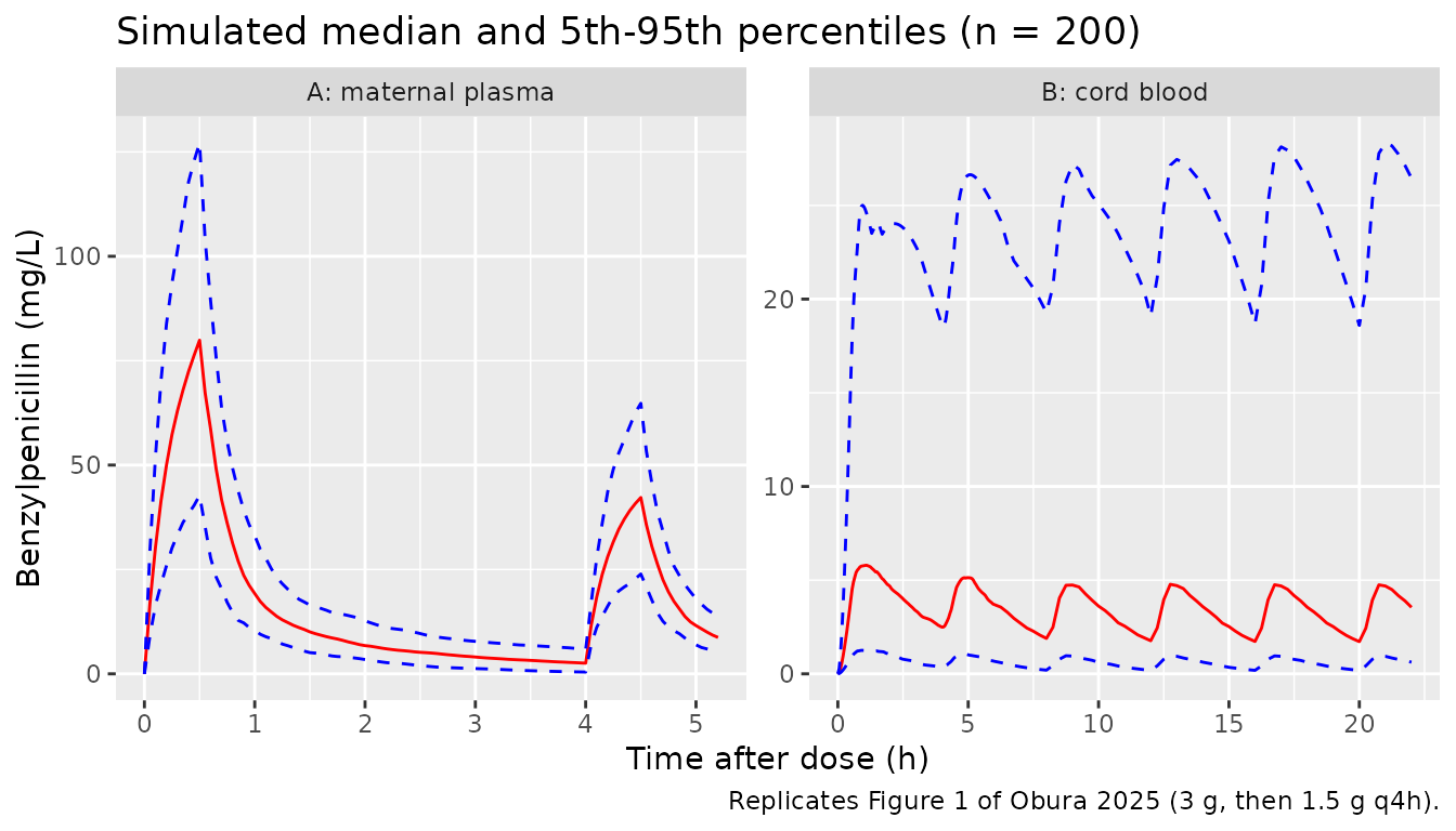
The trial regimen is a 3 g loading dose followed by 1.5 g every 4 h, each as a 0.5-h infusion. The Figure 1 visual predictive check plots time after the first dose, with maternal sampling over the first 4 h and one cord sample per woman at delivery (1-20 h). A cohort of 200 virtual women is given the loading dose and five maintenance doses (to 20 h). No covariates enter the model, so the cohort needs no covariate columns.
N_VPC <- 200
grid_vpc <- sort(unique(c(seq(0, 6, by = 0.05), seq(6, 22, by = 0.25))))
ev_vpc <- make_ev(3000, 1500, 0.5, grid_vpc, n = N_VPC)

rxode2::rxSetSeed(20250708)
sim_vpc <- rxode2::rxSolve(mod, events = ev_vpc, useLinCmt = FALSE) |>
  as.data.frame()
#> ℹ parameter labels from comments will be replaced by 'label()'

vpc <- sim_vpc |>
  dplyr::select(id, time, Cc, Ccord) |>
  tidyr::pivot_longer(c(Cc, Ccord), names_to = "matrix", values_to = "conc") |>
  dplyr::group_by(matrix, time) |>
  dplyr::summarise(
    p05 = quantile(conc, 0.05), p50 = median(conc), p95 = quantile(conc, 0.95),
    .groups = "drop"
  ) |>
  dplyr::mutate(
    matrix = dplyr::recode(matrix, Cc = "A: maternal plasma", Ccord = "B: cord blood")
  ) |>
  dplyr::filter(matrix == "B: cord blood" | time <= 5.2)

stopifnot(dplyr::n_distinct(sim_vpc$id) == N_VPC)
Replicate published figures
Figure 1 – visual predictive check
ggplot(vpc, aes(time)) +
  geom_line(aes(y = p50), colour = "red") +
  geom_line(aes(y = p05), colour = "blue", linetype = "dashed") +
  geom_line(aes(y = p95), colour = "blue", linetype = "dashed") +
  facet_wrap(~matrix, scales = "free") +
  labs(
    x = "Time after dose (h)", y = "Benzylpenicillin (mg/L)",
    title = "Simulated median and 5th-95th percentiles (n = 200)",
    caption = "Replicates Figure 1 of Obura 2025 (3 g, then 1.5 g q4h)."
  )
peak_time <- vpc |>
  dplyr::filter(matrix == "A: maternal plasma", time <= 1) |>
  dplyr::slice_max(p50, n = 1) |>
  dplyr::pull(time)
vpc |>
  dplyr::filter(
    matrix == "A: maternal plasma",
    sapply(time, function(t) any(abs(t - c(peak_time, 1, 2, 4)) < 1e-8))
  ) |>
  dplyr::select(time, p05, p50, p95) |>
  dplyr::rename(
    "Time after dose (h)" = time, "5th pctile (mg/L)" = p05,
    "Median (mg/L)" = p50, "95th pctile (mg/L)" = p95
  ) |>
knitr::kable(digits = 2, caption = "Simulated maternal percentiles after the 3 g loading dose (first row: median peak). Figure 1A: median about 80 mg/L at the 0.5-h peak with 5th-95th about 45-120 mg/L, falling to about 20-25 mg/L at 1 h and about 2-3 mg/L at 4 h; observed peaks 31-112 mg/L.")| Time after dose (h) | 5th pctile (mg/L) | Median (mg/L) | 95th pctile (mg/L) |
|---|---|---|---|
| 0.5 | 42.73 | 79.91 | 127.14 |
| 1.0 | 10.50 | 19.23 | 33.12 |
| 2.0 | 3.42 | 6.76 | 12.69 |
| 4.0 | 0.43 | 2.55 | 5.86 |
Figure 4 – simulated unbound profiles under four regimens
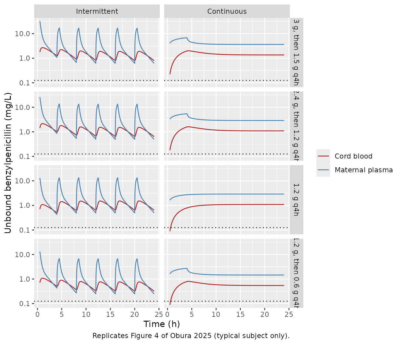
Figure 4 plots unbound plasma and cord concentrations for the four regimens, as intermittent (left) and continuous (right) infusions. The typical-subject profiles below reproduce the panel shapes; the dotted line is the 0.125 mg/L target.
grid_fig4 <- seq(0, 24, by = 0.05)
fig4 <- list()
for (i in seq_len(nrow(regimens))) {
  for (mode in c("Intermittent", "Continuous")) {
    dur <- if (mode == "Intermittent") 0.5 else 4
    s <- rxode2::rxSolve(
      mod_typ,
      events = make_ev(regimens$load[i], regimens$maint[i], dur, grid_fig4),
      useLinCmt = FALSE
    ) |>
      as.data.frame()
    fig4[[length(fig4) + 1]] <- tibble::tibble(
      regimen = regimens$regimen[i], mode = mode, time = s$time,
      `Maternal plasma` = FU * s$Cc, `Cord blood` = FU * s$Ccord
    )
  }
}
#> ℹ omega/sigma items treated as zero: 'etalcl', 'etalvc', 'etalk12', 'etalk21', 'etalk_central_cord', 'etalk_cord_central', 'etalvcord'
#> ℹ omega/sigma items treated as zero: 'etalcl', 'etalvc', 'etalk12', 'etalk21', 'etalk_central_cord', 'etalk_cord_central', 'etalvcord'
#> ℹ omega/sigma items treated as zero: 'etalcl', 'etalvc', 'etalk12', 'etalk21', 'etalk_central_cord', 'etalk_cord_central', 'etalvcord'
#> ℹ omega/sigma items treated as zero: 'etalcl', 'etalvc', 'etalk12', 'etalk21', 'etalk_central_cord', 'etalk_cord_central', 'etalvcord'
#> ℹ omega/sigma items treated as zero: 'etalcl', 'etalvc', 'etalk12', 'etalk21', 'etalk_central_cord', 'etalk_cord_central', 'etalvcord'
#> ℹ omega/sigma items treated as zero: 'etalcl', 'etalvc', 'etalk12', 'etalk21', 'etalk_central_cord', 'etalk_cord_central', 'etalvcord'
#> ℹ omega/sigma items treated as zero: 'etalcl', 'etalvc', 'etalk12', 'etalk21', 'etalk_central_cord', 'etalk_cord_central', 'etalvcord'
#> ℹ omega/sigma items treated as zero: 'etalcl', 'etalvc', 'etalk12', 'etalk21', 'etalk_central_cord', 'etalk_cord_central', 'etalvcord'
fig4 <- dplyr::bind_rows(fig4) |>
  tidyr::pivot_longer(c(`Maternal plasma`, `Cord blood`), names_to = "matrix", values_to = "fconc") |>
  dplyr::filter(time >= 0.5) |>
  dplyr::mutate(
    regimen = factor(regimen, levels = regimens$regimen),
    mode = factor(mode, levels = c("Intermittent", "Continuous"))
  )

ggplot(fig4, aes(time, fconc, colour = matrix)) +
  geom_hline(yintercept = MIC, linetype = "dotted") +
  geom_line() +
  facet_grid(regimen ~ mode) +
  scale_y_log10() +
  scale_colour_manual(values = c("Maternal plasma" = "steelblue", "Cord blood" = "firebrick")) +
  labs(
    x = "Time (h)", y = "Unbound benzylpenicillin (mg/L)", colour = NULL,
    caption = "Replicates Figure 4 of Obura 2025 (typical subject only)."
  )
Target attainment (Table 3)
The paper’s endpoint is the proportion of simulated women whose unbound concentration stays above 0.125 mg/L throughout the first 24 h, in plasma and in cord blood. Here 200 women per regimen are simulated with the packaged log-normal random effects, and the minimum unbound concentration is taken from the end of the first 0.5-h window to 24 h (Figure 4 also starts at 0.5 h).
N_PTA <- 200
grid_pta <- seq(0.5, 24, by = 0.1)
pta <- list()
rxode2::rxSetSeed(20250709)
for (i in seq_len(nrow(regimens))) {
  for (mode in c("Intermittent", "Continuous")) {
    dur <- if (mode == "Intermittent") 0.5 else 4
    ev <- make_ev(regimens$load[i], regimens$maint[i], dur, grid_pta, n = N_PTA)
    s <- as.data.frame(rxode2::rxSolve(mod, events = ev, useLinCmt = FALSE))
    per_id <- s |>
      dplyr::group_by(id) |>
      dplyr::summarise(fmin_plasma = FU * min(Cc), fmin_cord = FU * min(Ccord), .groups = "drop")
    pta[[length(pta) + 1]] <- tibble::tibble(
      regimen = regimens$regimen[i], mode = mode,
      pta_plasma = 100 * mean(per_id$fmin_plasma > MIC),
      pta_cord = 100 * mean(per_id$fmin_cord > MIC)
    )
  }
}
pta <- dplyr::bind_rows(pta)

table3 <- tibble::tribble(
  ~regimen,               ~mode,          ~ref_plasma, ~ref_cord,
  "3 g, then 1.5 g q4h",   "Intermittent", 95.82,       96.86,
  "2.4 g, then 1.2 g q4h", "Intermittent", 92.64,       93.92,
  "1.2 g q4h",             "Intermittent", 88.40,       83.5,
  "1.2 g, then 0.6 g q4h", "Intermittent", 69.16,       79.74,
  "3 g, then 1.5 g q4h",   "Continuous",   100,         74.8,
  "2.4 g, then 1.2 g q4h", "Continuous",   100,         68.44,
  "1.2 g q4h",             "Continuous",   100,         29.06,
  "1.2 g, then 0.6 g q4h", "Continuous",   100,         27.94
)

pta_cmp <- dplyr::inner_join(table3, pta, by = c("regimen", "mode"))

# Continuous infusion holds the unbound plasma concentration more than tenfold
# above the target for the typical woman under every regimen, so attainment is
# near-complete regardless of which subjects land in the tails.
stopifnot(all(pta_cmp$pta_plasma[pta_cmp$mode == "Continuous"] >= 95))

pta_cmp |>
  dplyr::select(regimen, mode, ref_plasma, pta_plasma, ref_cord, pta_cord) |>
  dplyr::rename(
    "Regimen" = regimen, "Infusion" = mode,
    "Table 3 plasma (%)" = ref_plasma, "Simulated plasma (%)" = pta_plasma,
    "Table 3 cord (%)" = ref_cord, "Simulated cord (%)" = pta_cord
  ) |>
knitr::kable(digits = 1, caption = "Probability of unbound Cmin > 0.125 mg/L over the first 24 h.")| Regimen | Infusion | Table 3 plasma (%) | Simulated plasma (%) | Table 3 cord (%) | Simulated cord (%) |
|---|---|---|---|---|---|
| 3 g, then 1.5 g q4h | Intermittent | 95.8 | 95.0 | 96.9 | 90.0 |
| 2.4 g, then 1.2 g q4h | Intermittent | 92.6 | 94.5 | 93.9 | 89.0 |
| 1.2 g q4h | Intermittent | 88.4 | 93.5 | 83.5 | 80.0 |
| 1.2 g, then 0.6 g q4h | Intermittent | 69.2 | 77.5 | 79.7 | 68.0 |
| 3 g, then 1.5 g q4h | Continuous | 100.0 | 100.0 | 74.8 | 65.0 |
| 2.4 g, then 1.2 g q4h | Continuous | 100.0 | 100.0 | 68.4 | 58.5 |
| 1.2 g q4h | Continuous | 100.0 | 100.0 | 29.1 | 38.5 |
| 1.2 g, then 0.6 g q4h | Continuous | 100.0 | 100.0 | 27.9 | 28.0 |
The simulated attainment reproduces the paper’s main conclusions: continuous infusion keeps plasma above target for essentially everyone, and lowering the intermittent regimen erodes plasma attainment, most sharply for 1.2 g then 0.6 g. It also reproduces the paper’s finding that cord attainment is lower under continuous than under intermittent infusion. Exact agreement with Table 3 is not expected. The paper sampled the NPAG support points with Pmetrics, truncating each parameter to between 0 and 3 times its observed maximum, and the timing window it used for the minimum is not stated; this vignette uses a log-normal approximation and a 0.5-24 h window. Cord attainment under continuous infusion is the most sensitive to that window, because the cord compartment fills slowly from zero.
PKNCA validation
Obura 2025 reports noncompartmental results for the observed maternal data after the first dose: peak 75.71 +/- 24.02 mg/L, AUC0-inf 87.88 +/- 27.41 mg*h/L and elimination half-life 0.54 h. Those come from the trial’s sampling schedule (before and 0.25, 0.5, 1, 2 and 4 h after the dose; the first maintenance dose follows at 4 h). The comparison below simulates 200 women given the 3 g loading dose as a single 0.5-h infusion and runs PKNCA twice on the same profiles: once on the trial schedule, which is the like-for-like comparison with the paper, and once on a dense 0-12 h grid. Per-subject results are averaged with the arithmetic mean, as the paper reports them.
N_NCA <- 200
TRIAL_TIMES <- c(0, 0.25, 0.5, 1, 2, 4)
grid_nca <- sort(unique(c(seq(0, 2, by = 0.05), seq(2, 12, by = 0.25), TRIAL_TIMES)))
ev_nca <- rxode2::et(amt = 3000, time = 0, dur = 0.5, cmt = "central") |>
  rxode2::et(grid_nca, cmt = "central") |>
  rxode2::et(id = seq_len(N_NCA)) |>
  as.data.frame()
ev_nca$dvid <- ifelse(ev_nca$evid == 0, 1L, NA_integer_)

rxode2::rxSetSeed(20250710)
sim_dense <- rxode2::rxSolve(mod, events = ev_nca, useLinCmt = FALSE) |>
  as.data.frame() |>
  dplyr::filter(!is.na(Cc)) |>
  dplyr::select(id, time, Cc)

# Time-zero anchor for AUC0-inf.
sim_dense <- dplyr::bind_rows(
  sim_dense,
  sim_dense |> dplyr::distinct(id) |> dplyr::mutate(time = 0, Cc = 0)
) |>
  dplyr::distinct(id, time, .keep_all = TRUE) |>
  dplyr::arrange(id, time)

sim_nca <- dplyr::bind_rows(
  sim_dense |> dplyr::mutate(sampling = "Dense 0-12 h"),
  sim_dense |>
    dplyr::filter(sapply(time, function(t) any(abs(t - TRIAL_TIMES) < 1e-8))) |>
    dplyr::mutate(sampling = "Trial schedule 0-4 h")
)
stopifnot(all(table(sim_nca$sampling[sim_nca$id == 1]) >= length(TRIAL_TIMES)))

dose_df <- sim_nca |>
  dplyr::distinct(id, sampling) |>
  dplyr::mutate(time = 0, amt = 3000)

conc_obj <- PKNCA::PKNCAconc(sim_nca, Cc ~ time | sampling + id)
dose_obj <- PKNCA::PKNCAdose(dose_df, amt ~ time | sampling + id)
intervals <- data.frame(
  start = 0, end = Inf, cmax = TRUE, tmax = TRUE, aucinf.obs = TRUE, half.life = TRUE
)
nca_res <- PKNCA::pk.nca(PKNCA::PKNCAdata(conc_obj, dose_obj, intervals = intervals))

nca_mean <- as.data.frame(nca_res$result) |>
  dplyr::filter(PPTESTCD %in% c("cmax", "aucinf.obs", "half.life")) |>
  dplyr::group_by(sampling, PPTESTCD) |>
  dplyr::summarise(PPORRES = mean(PPORRES, na.rm = TRUE), .groups = "drop")

reference <- data.frame(
  sampling = c("Trial schedule 0-4 h", "Dense 0-12 h"),
  cmax = 75.71, aucinf.obs = 87.88, half.life = 0.54
)

cmp_nca <- nlmixr2lib::ncaComparisonTable(
  simulated = nca_mean,
  reference = reference,
  by = "sampling",
  units = c(cmax = "mg/L", aucinf.obs = "mg*h/L", half.life = "h"),
  tolerance_pct = 20
)
knitr::kable(cmp_nca, caption = "Simulated mean NCA vs Obura 2025 Results (observed data, first dose).")| NCA parameter | sampling | Reference | Simulated | % diff |
|---|---|---|---|---|
| Cmax (mg/L) | Trial schedule 0-4 h | 75.7 | 78.7 | +3.9% |
| Cmax (mg/L) | Dense 0-12 h | 75.7 | 78.7 | +3.9% |
| AUC0-∞ (obs) (mg*h/L) | Trial schedule 0-4 h | 87.9 | 73.4 | -16.5% |
| AUC0-∞ (obs) (mg*h/L) | Dense 0-12 h | 87.9 | 74.3 | -15.4% |
| t½ (h) | Trial schedule 0-4 h | 0.54 | 1.33 | +146.6%* |
| t½ (h) | Dense 0-12 h | 0.54 | 2.16 | +300.4%* |
# AUC0-inf of a linear model is dose / CL for every subject, whatever the
# distribution kinetics, so the dense-grid population mean is fixed by CL and
# its variance alone.
nca_val <- function(smp, code) {
  nca_mean$PPORRES[nca_mean$sampling == smp & nca_mean$PPTESTCD == code]
}
auc_typ <- 3000 / exp(ui$theta[["lcl"]])
auc_dense <- nca_val("Dense 0-12 h", "aucinf.obs")
stopifnot(abs(auc_dense / (auc_typ * exp(ui$omega["etalcl", "etalcl"] / 2)) - 1) < 0.1)

# Three-exponential disposition of the typical woman: the eigenvalues of the
# rate matrix of Equations 4-6.
th <- exp(ui$theta)
kmat <- with(as.list(th), matrix(c(
  -(lcl / lvc + lk12 + lk_central_cord), lk21, lk_cord_central,
  lk12, -lk21, 0,
  lk_central_cord, 0, -lk_cord_central
), nrow = 3, byrow = TRUE))
half_lives <- sort(log(2) / -eigen(kmat)$values)
tibble::tibble(
  quantity = c(
    "Typical dose / CL (mg*h/L)", "Dense-grid mean AUC0-inf (mg*h/L)",
    "Trial-schedule mean AUC0-inf (mg*h/L)",
    "Disposition half-lives of the typical woman (h)"
  ),
  value = c(
    sprintf("%.1f", auc_typ), sprintf("%.1f", auc_dense),
    sprintf("%.1f", nca_val("Trial schedule 0-4 h", "aucinf.obs")),
    paste(sprintf("%.2f", half_lives), collapse = ", ")
  )
) |>
  dplyr::rename("Quantity" = quantity, "Value" = value) |>
knitr::kable(caption = "Closed-form checks behind the NCA comparison.")| Quantity | Value |
|---|---|
| Typical dose / CL (mg*h/L) | 72.7 |
| Dense-grid mean AUC0-inf (mg*h/L) | 74.3 |
| Trial-schedule mean AUC0-inf (mg*h/L) | 73.4 |
| Disposition half-lives of the typical woman (h) | 0.15, 1.15, 1.55 |
The simulated mean peak matches the paper’s NCA. The half-life does not, on either grid, and it is a property of the sampling window rather than of the encoding: the typical woman’s disposition has three phases (half-lives above), the PKNCA lambda-z search on the trial schedule spans 1-4 h and lands between the second and third, and a dense grid reaching 12 h finds the slow terminal phase. The paper’s 0.54 h is closer to the 1-2 h decline alone (the simulated median falls from about 19 to about 7 mg/L over that hour, a half-life of about 0.7 h), and the paper does not state which samples it used. The simulated percentiles track the Figure 1A visual predictive check at 1, 2 and 4 h (see the Figure 1 table), which is the model’s own description of the same data. AUC0-inf is fixed by the model’s mean clearance (dose / CL = 72.7 mgh/L for the typical woman), so the simulated mean lies below the observed 87.88 mgh/L; that gap reflects the difference between the observed NCA of 12 women and the NPAG clearance estimate, not an encoding error.
Assumptions and deviations
- Typical values are the Table 2 means. NPAG’s joint distribution has both a weighted mean and a median; the means are the values quoted in the Abstract and the Results, and a typical-value solve with them reproduces Table S1 and the Figure 4 cord plateau much better than the medians do (see “Which Table 2 column is the typical value”).
-
Inter-individual variability is a log-normal
approximation. NPAG estimates a discrete distribution on 12
support points, whose shape is not published. Each parameter’s variance
is
log(1 + CV^2)from the Table 2 CV, and the Table 2 CL-Vc correlation of 0.67 (a correlation of the support points on the linear scale) is used as the correlation ofetalclandetalvc. No other correlations are reported, so the other etas are independent. -
Residual error. Pmetrics weights each observation
by an assay SD polynomial, here
SD = 0.1 + 0.02 x C, multiplied by the fitted gamma of 4.72. That is a linear sum of an additive and a proportional term, encoded ascombined1()withaddSd = 0.472mg/L andpropSd = 0.0944. Pmetrics evaluates the polynomial at the observed concentration; nlmixr2 evaluates it at the prediction. Data S1 Text S2 lists one gamma with the same polynomial for both outputs, so the cord residual error has the same values. -
The cord compartment returns drug to the mother.
Equations 4-6 make the cord compartment a reversible distribution space
with no elimination of its own. It is named
cord, following the umbilical cord compartment ofNie_2025_sufentanil, and declared throughpaper_specific_compartments. - Protein binding is not part of the model. Concentrations are total drug. The 60% protein binding (unbound fraction 0.4) that the paper uses for target attainment is applied in this vignette only.
- Continuous-infusion schedule. The paper does not spell out how its continuous-infusion versions of the loading-plus-maintenance regimens were delivered. Each dose is infused over its whole 4-h interval here, which reproduces both Table S1 (continuous-infusion AUC equal to the intermittent AUC) and the shape of Figure 4.
- Target-attainment window. The minimum unbound concentration is taken over 0.5-24 h; the paper’s exact window is not stated.
- Figure 4 plateau values (plasma about 3.6 mg/L, cord about 1.35 mg/L unbound) were read off the plot by the maintainers and are used only as a check; no model parameter is derived from them.
- NCA half-life and AUC. The paper’s observed-data NCA half-life (0.54 h) and mean AUC0-inf (87.88 mg*h/L) are not reproduced: the simulated trial-schedule values are about 1.3 h and 15% lower (see “PKNCA validation”). The AUC is fixed by the Table 2 mean clearance and the half-life by the lambda-z window, which the paper does not report; no parameter was adjusted.
- No erratum for Obura 2025 was found on Europe PMC (checked 2026-11-06).