Infliximab (Ternant 2021)

library(nlmixr2lib)
library(PKNCA)
#> 
#> Attaching package: 'PKNCA'
#> The following object is masked from 'package:stats':
#> 
#>     filter
library(rxode2)
#> rxode2 5.1.8 using 2 threads (see ?getRxThreads)
#>   no cache: create with `rxCreateCache()`
library(dplyr)
#> 
#> Attaching package: 'dplyr'
#> The following objects are masked from 'package:stats':
#> 
#>     filter, lag
#> The following objects are masked from 'package:base':
#> 
#>     intersect, setdiff, setequal, union
library(tidyr)
library(ggplot2)

Model and source

• Citation: Ternant D, Le Tilly O, Picon L, Moussata D, Passot C, Bejan-Angoulvant T, Desvignes C, Mulleman D, Goupille P, Paintaud G. Infliximab Efficacy May Be Linked to Full TNF-alpha Blockade in Peripheral Compartment - A Double Central-Peripheral Target-Mediated Drug Disposition (TMDD) Model. Pharmaceutics. 2021;13(11):1821. doi:10.3390/pharmaceutics13111821
• Description: Two-compartment population PK model of intravenous infliximab with double quasi-steady-state (QSS) target-mediated drug disposition (TMDD): infliximab binds TNF-alpha in both the central and the peripheral compartment, each with its own baseline target level, steady-state dissociation constant and complex elimination rate, and a shared fixed TNF-alpha elimination rate. Fitted jointly to adults with inflammatory bowel disease (Crohn’s disease or ulcerative colitis; TMDD active) and adults with ankylosing spondylitis (linear reference with no target interaction). Covariates: body weight and sex on V1, sex on CL, ulcerative colitis on central baseline TNF-alpha (Ternant 2021).
• Article: https://doi.org/10.3390/pharmaceutics13111821
• Supplement: https://www.mdpi.com/article/10.3390/pharmaceutics13111821/s1

Ternant et al. (2021) extended a two-compartment infliximab model with target-mediated drug disposition (TMDD) in both compartments. Infliximab binds TNF-alpha in the central compartment and, separately, in the peripheral compartment. Each pool has its own baseline level (R0), steady-state dissociation constant (KSS) and complex elimination rate (kint). The two pools share one TNF-alpha elimination rate (kout), which could not be estimated and was fixed at 20 1/day. Binding uses the quasi-steady-state (QSS) approximation.

The model was fitted jointly to two cohorts. The ankylosing spondylitis (AS) patients were the linear-kinetics reference: for them the target-mediated terms are switched off and the target states start at zero. The inflammatory bowel disease (IBD) patients had the TMDD terms switched on. The switch is written into the published Monolix code (Appendix A, regressors IBD and DIS). Here it is rebuilt from the two canonical disease indicators as IBD = DIS_CD + DIS_UC, so a subject with both indicators at 0 is an AS reference patient.

Population

The analysis pooled 158 adults from two French cohorts (Table 1):

• IBD cohort (n = 133): a retrospective routine-care cohort at Tours University Hospital (2006-2012). There were 108 patients with Crohn’s disease and 25 with ulcerative colitis, 53 female and 80 male. Median age was 34 years (IQR 25-41) and median body weight 64 kg (IQR 56-72). They received 5 mg/kg infliximab at weeks 0, 2 and 6, then every 8 weeks, and contributed 845 trough and peak concentrations.
• AS cohort (n = 25; SPAXIM trial, NCT00607403): 6 female and 19 male. Median age was 43 years (IQR 35-52) and median body weight 75 kg (IQR 65-85). They received 5 mg/kg at weeks 0, 2, 6, 12 and 18 with dense sampling, which gave 488 concentrations.

The ELISA measures unbound infliximab (LLOQ 0.103 mg/L). IBD cycles with detectable anti-drug antibodies were discarded.

The same information is available programmatically via rxode2::rxode2(readModelDb("Ternant_2021_infliximab"))$population.

Source trace

Every ini() value carries a source comment in inst/modeldb/specificDrugs/Ternant_2021_infliximab.R. The table below collects them in one place.

Equation / parameter	Value	Source location
lcl (CL, female)	log(0.16) L/day	Table 2, final model
lvc (V1, female, 65 kg)	log(2.6) L	Table 2, final model
lvp (V2)	log(1.9) L	Table 2, final model
lq (Q)	log(1.8) L/day	Table 2, final model
lkss (KSS_C)	log(15.4) nM	Table 2, final model
lrbase_target (R0_C, Crohn’s disease)	log(3.3) nM	Table 2, final model
lkint (kint_C)	log(0.17) 1/day	Table 2, final model
lkss_peripheral1 (KSS_P)	log(0.49) nM	Table 2, final model
lrbase_target_peripheral1 (R0_P)	log(0.46) nM	Table 2, final model
lkint_peripheral1 (kint_P)	log(0.0079) 1/day	Table 2, final model
lkdeg (kout, both compartments)	fixed(log(20)) 1/day	Table 2; Results 3.1; Supplement Table S1
e_wt_vc	0.33	Table 2 BW_V1
e_sexmale_vc	0.13	Table 2 SX_V1
e_sexmale_cl	0.36	Table 2 SX_CL; Results 3.2 (CL in males 0.23 L/day)
e_dis_uc_rbase_target	0.57	Table 2 UC_RC0; Results 3.2 (R0_C in UC 5.8 nM)
etalvc, etalcl, etalvp	0.27^2, 0.35^2, 0.39^2	Table 2 omega (SD)
etalrbase_target, etalrbase_target_peripheral1	1.0^2, 1.1^2	Table 2 omega (SD)
addSd, propSd	1.8 mg/L, 0.20	Table 2 sigma; Methods 2.2.2 (mixed additive-proportional)
Covariate forms	ln(theta) = ln(theta_ref) + beta * CAT; power weight centred on median	Methods 2.2.2
d/dt(central), d/dt(peripheral1)	n/a	Methods 2.2.1 equations; Appendix A ddt_CT, ddt_CP
d/dt(total_target), d/dt(total_target_peripheral1)	n/a	Methods 2.2.1 equations; Appendix A ddt_cRT, ddt_pRT
QSS unbound drug cfree, cfree_peripheral1	n/a	Methods 2.2.1 equations; Appendix A cINTER, cDELTA, Cf, Cp
Target initial conditions R0 * IBD	n/a	Appendix A cRT_0, pRT_0
mg to nM conversion, 1 nM = 0.1442 mg/L	n/a	Appendix A iv(p=(1/0.144200)/V1), Cc = Cf*0.144200

The states hold total infliximab amounts in mg. The Monolix code instead integrates concentrations in nM, and its peripheral equation (ddt_CP = k12*Cf - k21*Cp) refers the peripheral concentration to V1, not V2. The model file converts central / vc and peripheral1 / vc to nM in the same way, so the QSS algebra matches the published code term for term. Only the dosing entry point differs.

Virtual cohort

The simulation follows the paper’s own set-up (Methods 2.3):

• 5 mg/kg infused at weeks 0, 2, 6, 14 and 22 (2-hour infusions);
• male:female 50:50 and Crohn’s disease:ulcerative colitis 5:1;
• body weight normal with mean 66 kg and SD 15 kg, restricted to the population range 41-110 kg.

# rxode2's RNG stream depends on the solver thread count, so the cohort drawn
# here is not identical across machines. Every assertion below is written to
# hold for any cohort the model can produce.
set.seed(20211101)
rxode2::rxSetSeed(20211101)

n_ibd <- 200L
dose_days <- c(0, 2, 6, 14, 22) * 7
inf_dur <- 2 / 24 # 2-hour infusion, in days

draw_wt <- function(n) {
  out <- numeric(0)
  while (length(out) < n) {
    x <- rnorm(n, 66, 15)
    out <- c(out, x[x >= 41 & x <= 110])
  }
  out[seq_len(n)]
}

subjects <- tibble(
  id = seq_len(n_ibd),
  WT = draw_wt(n_ibd),
  SEXF = rbinom(n_ibd, 1, 0.5),
  DIS_UC = rbinom(n_ibd, 1, 1 / 6)
) |>
  mutate(
    DIS_CD = 1L - DIS_UC,
    disease = ifelse(DIS_UC == 1, "Ulcerative colitis", "Crohn's disease")
  )

# Observe on a half-day grid plus just before each infusion (exact troughs) and
# at the end of each infusion (exact peaks).
obs_times <- sort(unique(c(
  seq(0, 160, by = 0.5), dose_days[-1] - 0.01, dose_days + inf_dur
)))

doses <- subjects |>
  tidyr::crossing(time = dose_days) |>
  mutate(evid = 1L, amt = 5 * WT, dur = inf_dur, cmt = "central")
obs <- subjects |>
  tidyr::crossing(time = obs_times) |>
  mutate(evid = 0L, amt = 0, dur = 0, cmt = "central")
events <- bind_rows(doses, obs) |>
  arrange(id, time, desc(evid)) |>
  as.data.frame()

stopifnot(
  !anyDuplicated(events[, c("id", "time", "evid")]),
  nrow(subjects) == n_ibd
)

Simulation

mod <- readModelDb("Ternant_2021_infliximab")

sim <- rxode2::rxSolve(
  mod,
  events = events,
  keep = c("disease", "WT", "SEXF"),
  returnType = "data.frame"
) |>
  mutate(
    ratio_central = target_free / total_target,
    ratio_peripheral = target_free_peripheral1 / total_target_peripheral1
  )
#> ℹ parameter labels from comments will be replaced by 'label()'

Replicate Figure 3

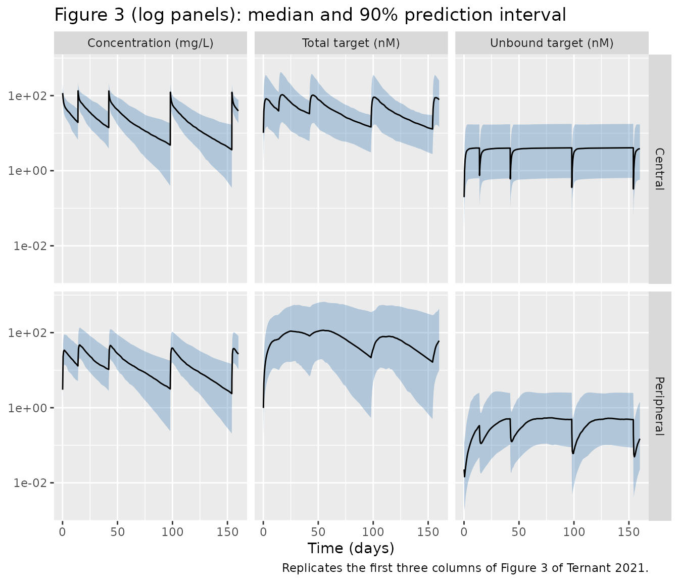
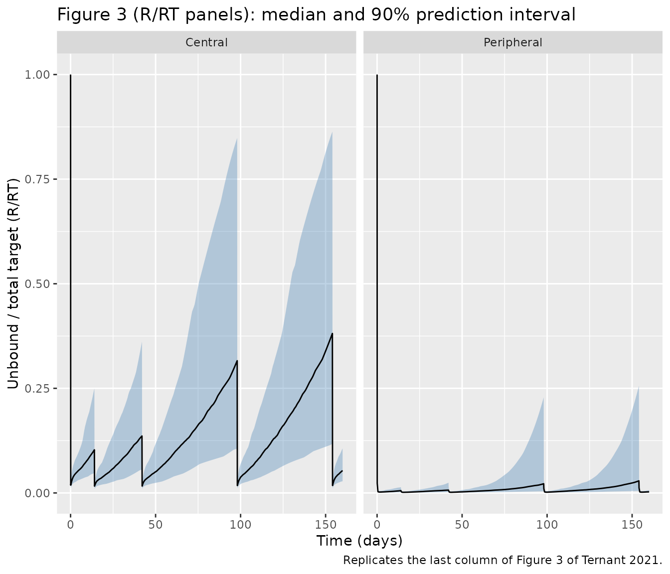
Figure 3 of the paper shows the median and 90% prediction interval of four quantities in each compartment: infliximab concentration, total target, unbound target, and the unbound/total target ratio R/RT. The simulated equivalents are below. The central infliximab concentration is the observed unbound serum concentration Cc. The peripheral concentration is the unbound peripheral drug on the same mg/L scale (cfree_peripheral1 * 0.1442).

fig3 <- sim |>
  mutate(Cc_peripheral = cfree_peripheral1 * 0.1442) |>
  select(
    id, time,
    `Central|Concentration (mg/L)` = Cc,
    `Central|Total target (nM)` = total_target,
    `Central|Unbound target (nM)` = target_free,
    `Central|R/RT` = ratio_central,
    `Peripheral|Concentration (mg/L)` = Cc_peripheral,
    `Peripheral|Total target (nM)` = total_target_peripheral1,
    `Peripheral|Unbound target (nM)` = target_free_peripheral1,
    `Peripheral|R/RT` = ratio_peripheral
  ) |>
  pivot_longer(-c(id, time), names_to = "key", values_to = "value") |>
  separate(key, into = c("compartment", "quantity"), sep = "\\|") |>
  group_by(compartment, quantity, time) |>
  summarise(
    Q05 = quantile(value, 0.05, na.rm = TRUE),
    Q50 = quantile(value, 0.50, na.rm = TRUE),
    Q95 = quantile(value, 0.95, na.rm = TRUE),
    .groups = "drop"
  ) |>
  mutate(quantity = factor(quantity, levels = c(
    "Concentration (mg/L)", "Total target (nM)", "Unbound target (nM)", "R/RT"
  )))

log_panels <- fig3 |> filter(quantity != "R/RT", time > 0)
ggplot(log_panels, aes(time, Q50)) +
  geom_ribbon(aes(ymin = Q05, ymax = Q95), fill = "steelblue", alpha = 0.35) +
  geom_line() +
  facet_grid(compartment ~ quantity) +
  scale_y_log10() +
  labs(
    x = "Time (days)", y = NULL,
    title = "Figure 3 (log panels): median and 90% prediction interval",
    caption = "Replicates the first three columns of Figure 3 of Ternant 2021."
  )

ggplot(filter(fig3, quantity == "R/RT"), aes(time, Q50)) +
  geom_ribbon(aes(ymin = Q05, ymax = Q95), fill = "steelblue", alpha = 0.35) +
  geom_line() +
  facet_wrap(~compartment) +
  coord_cartesian(ylim = c(0, 1)) +
  labs(
    x = "Time (days)", y = "Unbound / total target (R/RT)",
    title = "Figure 3 (R/RT panels): median and 90% prediction interval",
    caption = "Replicates the last column of Figure 3 of Ternant 2021."
  )

Quantitative checks against the text of Results 3.3

Results 3.3 makes three numerical claims about these simulations:

1. before the third and fourth infusions the median central R/RT rises again (the paper says above 30%), while the median peripheral R/RT stays below 3%;
2. an infliximab serum concentration of 5 mg/L goes with median central and peripheral R/RT of 26% and 1.2%;
3. total target reaches 10- to 100-fold its baseline.

Under the QSS approximation the central ratio is not a free quantity. From Cf * R = KSS * (CT - Cf), the unbound/total target ratio is R/RT = KSS_C / (KSS_C + Cf) exactly, where Cf is unbound infliximab in nM. Claim 2 can therefore be checked without any simulation. The chunk below first confirms that the solved model obeys this identity, then evaluates it at 5 mg/L.

# Exact QSS identity for the central compartment, on every simulated row
# after the first dose. Both sides use the same solved state, so the
# difference is floating-point only.
kss_c <- exp(rxode2::rxode2(mod)$theta[["lkss"]])
#> ℹ parameter labels from comments will be replaced by 'label()'
post <- sim |> filter(time > 0)
identity_err <- max(abs(post$ratio_central - kss_c / (kss_c + post$cfree)))
identity_err
#> [1] 1.593291e-13

ratio_at <- function(cc_mgl) kss_c / (kss_c + cc_mgl / 0.1442)
c(ratio_at_5_mgL = ratio_at(5), conc_for_26pct_mgL = 0.1442 * kss_c * (1 / 0.26 - 1))
#>     ratio_at_5_mgL conc_for_26pct_mgL 
#>          0.3075444          6.3203969

troughs <- sim |>
  filter(time %in% (dose_days[3:4] - 0.01)) |>
  group_by(time) |>
  summarise(
    median_ratio_central = median(ratio_central),
    median_ratio_peripheral = median(ratio_peripheral),
    median_Cc = median(Cc),
    .groups = "drop"
  ) |>
  mutate(before_infusion = c("third (week 6)", "fourth (week 14)"))

at5 <- sim |>
  filter(time > 0, Cc >= 4.5, Cc <= 5.5) |>
  summarise(
    n_samples = n(),
    median_ratio_central = median(ratio_central),
    median_ratio_peripheral = median(ratio_peripheral)
  )

fold <- sim |>
  group_by(id) |>
  summarise(
    fold_central = max(total_target) / first(total_target),
    fold_peripheral = max(total_target_peripheral1) / first(total_target_peripheral1),
    .groups = "drop"
  )

troughs |>
  select(before_infusion, median_Cc, median_ratio_central, median_ratio_peripheral) |>
  dplyr::rename(
    "Before infusion" = before_infusion,
    "Median Cc (mg/L)" = median_Cc,
    "Median central R/RT" = median_ratio_central,
    "Median peripheral R/RT" = median_ratio_peripheral
  ) |>
  knitr::kable(digits = 3, caption = "Median target ratios at the pre-infusion troughs.")

Median target ratios at the pre-infusion troughs.

Before infusion	Median Cc (mg/L)	Median central R/RT	Median peripheral R/RT
third (week 6)	14.104	0.136	0.007
fourth (week 14)	4.812	0.316	0.022

at5 |>
  dplyr::rename(
    "Samples with Cc in 4.5-5.5 mg/L" = n_samples,
    "Median central R/RT (paper 0.26)" = median_ratio_central,
    "Median peripheral R/RT (paper 0.012)" = median_ratio_peripheral
  ) |>
  knitr::kable(digits = 3, caption = "Target ratios at an infliximab concentration of about 5 mg/L.")

Target ratios at an infliximab concentration of about 5 mg/L.

Samples with Cc in 4.5-5.5 mg/L	Median central R/RT (paper 0.26)	Median peripheral R/RT (paper 0.012)
1858	0.308	0.018

fold |>
  summarise(
    median_fold_central = median(fold_central),
    median_fold_peripheral = median(fold_peripheral)
  ) |>
  dplyr::rename(
    "Median max/baseline, central" = median_fold_central,
    "Median max/baseline, peripheral" = median_fold_peripheral
  ) |>
  knitr::kable(digits = 1, caption = "Peak total target relative to baseline.")

Peak total target relative to baseline.

Median max/baseline, central	Median max/baseline, peripheral
24.5	271.8

# The cohort gates below are on medians, never on cohort extremes.
# A mis-transcribed KSS, R0 or kint moves these ratios several-fold, so the
# bounds still catch structural errors. Measured at 200 subjects on the
# authoring machine: central 0.308 and peripheral 0.018 in the 4.5-5.5 mg/L
# bin; peripheral trough medians 0.007 and 0.022; central trough medians
# 0.14 and 0.32; fold medians 24 (central) and 270 (peripheral).
stopifnot(
  identity_err < 1e-8,
  # The 4.5-5.5 mg/L bin brackets the identity value 0.308 (0.286-0.330).
  abs(at5$median_ratio_central - ratio_at(5)) < 0.02,
  at5$median_ratio_peripheral > 0.005,
  at5$median_ratio_peripheral < 0.04,
  all(troughs$median_ratio_peripheral < 0.04),
  troughs$median_ratio_central[2] > 0.2,
  troughs$median_ratio_central[2] < 0.45,
  median(fold$fold_central) > 10,
  median(fold$fold_central) < 100,
  median(fold$fold_peripheral) > 50
)

Claim 1. Before the fourth infusion the median central R/RT is about 32%, in line with “above 30%”. Before the third infusion it is about 14%, which matches the lower peak of the Figure 3 ribbon at day 42. The median peripheral R/RT stays below 3% at both troughs, as stated.

Claim 2 (known deviation). With the paper’s own central KSS of 15.4 nM, the QSS identity gives a central R/RT of 30.8% at 5 mg/L (34.7 nM). A ratio of 26% would need about 6.3 mg/L. The simulated median in the 4.5-5.5 mg/L bin reproduces the identity, not the 26% in the text. The peripheral median is about 1.8% versus 1.2% in the text. The peripheral ratio depends on peripheral, not serum, concentrations, so it has no closed form. Both statements in the text fit better at a serum concentration of about 6 mg/L. The model is not adjusted to match them.

Claim 3. Peak central total target is about 24-fold baseline, inside the stated 10- to 100-fold range. Peak peripheral total target is about 272-fold its 0.46 nM baseline. That is above the stated range, but it agrees with Figure 3 itself: the median peripheral total target there rises from below 1 nM to about 100 nM.

Linear reference (ankylosing spondylitis): closed-form check

With both disease indicators at 0 the model must reduce to a plain linear two-compartment model with infusion input. Below, a typical AS patient is compared against the closed-form biexponential infusion solution computed from the same CL, V1, V2 and Q. The two sides share every parameter, so the difference is pure integration error and a tight bound is correct.

p <- rxode2::rxode2(mod)$theta
#> ℹ parameter labels from comments will be replaced by 'label()'
as_pat <- tibble(id = 1L, WT = 65, SEXF = 1, DIS_CD = 0, DIS_UC = 0)
as_ev <- bind_rows(
  as_pat |> tidyr::crossing(time = dose_days) |>
    mutate(evid = 1L, amt = 5 * WT, dur = inf_dur, cmt = "central"),
  as_pat |> tidyr::crossing(time = seq(0.5, 160, by = 0.5)) |>
    mutate(evid = 0L, amt = 0, dur = 0, cmt = "central")
) |>
  arrange(time, desc(evid)) |>
  as.data.frame()

as_sim <- rxode2::rxSolve(
  rxode2::zeroRe(mod), events = as_ev, returnType = "data.frame",
  rtol = 1e-10, atol = 1e-12
)
#> ℹ parameter labels from comments will be replaced by 'label()'
#> ℹ omega/sigma items treated as zero: 'etalvc', 'etalcl', 'etalvp', 'etalrbase_target', 'etalrbase_target_peripheral1'

two_cmt_infusion <- function(t, dose_times, amt, dur, cl, v1, v2, q) {
  k10 <- cl / v1; k12 <- q / v1; k21 <- q / v2
  s <- k10 + k12 + k21
  alpha <- (s + sqrt(s^2 - 4 * k10 * k21)) / 2
  beta <- (s - sqrt(s^2 - 4 * k10 * k21)) / 2
  a <- (alpha - k21) / (v1 * (alpha - beta))
  b <- (k21 - beta) / (v1 * (alpha - beta))
  rate <- amt / dur
  one <- function(tt) {
    ifelse(
      tt <= 0, 0,
      ifelse(
        tt <= dur,
        rate * (a / alpha * (1 - exp(-alpha * tt)) + b / beta * (1 - exp(-beta * tt))),
        rate * (a / alpha * (1 - exp(-alpha * dur)) * exp(-alpha * (tt - dur)) +
          b / beta * (1 - exp(-beta * dur)) * exp(-beta * (tt - dur)))
      )
    )
  }
  Reduce(`+`, lapply(dose_times, function(d) one(t - d)))
}

closed <- two_cmt_infusion(
  as_sim$time, dose_days, amt = 5 * 65, dur = inf_dur,
  cl = exp(p[["lcl"]]), v1 = exp(p[["lvc"]]), v2 = exp(p[["lvp"]]), q = exp(p[["lq"]])
)
rel_err <- max(abs(as_sim$Cc / closed - 1))
rel_err
#> [1] 5.677335e-10
stopifnot(
  rel_err < 1e-5,
  all(as_sim$total_target == 0),
  all(as_sim$total_target_peripheral1 == 0)
)

Terminal (non-target-mediated) half-life

Results 3.1 reports an endogenous, non-target-mediated elimination half-life of about 17 days. It follows from the individual linear parameters as log(2) / beta, where beta is the slow disposition eigenvalue.

hl <- sim |>
  distinct(id, SEXF, cl, vc, vp, q) |>
  mutate(
    k10 = cl / vc, k12 = q / vc, k21 = q / vp,
    s = k10 + k12 + k21,
    beta = (s - sqrt(s^2 - 4 * k10 * k21)) / 2,
    t_half_beta = log(2) / beta
  )

hl |>
  mutate(sex = ifelse(SEXF == 1, "Female", "Male")) |>
  group_by(sex) |>
  summarise(median_t_half_beta = median(t_half_beta), .groups = "drop") |>
  bind_rows(tibble(sex = "All", median_t_half_beta = median(hl$t_half_beta))) |>
  dplyr::rename(
    "Sex" = sex,
    "Median beta half-life (days)" = median_t_half_beta
  ) |>
  knitr::kable(digits = 1, caption = "Linear terminal half-life; paper value about 17 days.")

Linear terminal half-life; paper value about 17 days.

Sex	Median beta half-life (days)
Female	19.9
Male	16.2
All	18.3

stopifnot(abs(median(hl$t_half_beta) / 17 - 1) < 0.2)

The cohort median is about 18.3 days. Women (the CL and V1 reference) are near 20 days and men near 16 days. Averaged over the 50:50 simulated sex mix, this is close to the paper’s “approximately 17 days”.

PKNCA validation

The paper reports no NCA table. PKNCA is run on the simulated unbound serum concentrations for two intervals, grouped by disease: the first dosing interval (days 0-14) and the maintenance interval between the week-14 and week-22 infusions. The trough before week 22 can be compared with the 3-5 mg/L therapeutic target cited in the Introduction.

conc_nca <- sim |>
  filter(!is.na(Cc)) |>
  select(id, time, Cc, disease)
conc_nca <- bind_rows(
  conc_nca,
  conc_nca |> distinct(id, disease) |> mutate(time = 0, Cc = 0)
) |>
  distinct(id, disease, time, .keep_all = TRUE) |>
  arrange(id, disease, time)

dose_nca <- events |>
  filter(evid == 1) |>
  select(id, time, amt, disease)

conc_obj <- PKNCA::PKNCAconc(conc_nca, Cc ~ time | disease + id)
dose_obj <- PKNCA::PKNCAdose(dose_nca, amt ~ time | disease + id)

intervals <- data.frame(
  start = c(0, 98),
  end = c(14, 153.99),
  cmax = TRUE,
  tmax = TRUE,
  # The first interval starts at the pre-dose zero, so its minimum is not a
  # trough; Cmin is only requested for the maintenance interval.
  cmin = c(FALSE, TRUE),
  auclast = TRUE
)

nca_res <- PKNCA::pk.nca(PKNCA::PKNCAdata(conc_obj, dose_obj, intervals = intervals))

nca_tab <- as.data.frame(nca_res) |>
  filter(PPTESTCD %in% c("cmax", "tmax", "cmin", "auclast")) |>
  group_by(disease, start, PPTESTCD) |>
  summarise(median = median(PPORRES, na.rm = TRUE), .groups = "drop") |>
  pivot_wider(names_from = PPTESTCD, values_from = median) |>
  mutate(interval = ifelse(start == 0, "Days 0-14", "Weeks 14-22")) |>
  select(disease, interval, cmax, tmax, cmin, auclast)

nca_tab |>
  dplyr::rename(
    "Disease" = disease,
    "Interval" = interval,
    "Cmax (mg/L)" = cmax,
    "Tmax (day)" = tmax,
    "Cmin (mg/L)" = cmin,
    "AUClast (mg*day/L)" = auclast
  ) |>
  knitr::kable(digits = 2, caption = "Median simulated NCA parameters by disease.")

Median simulated NCA parameters by disease.

Disease	Interval	Cmax (mg/L)	Tmax (day)	Cmin (mg/L)	AUClast (mg*day/L)
Crohn’s disease	Days 0-14	114.78	0.08	NA	515.37
Crohn’s disease	Weeks 14-22	122.45	0.08	3.69	1004.64
Ulcerative colitis	Days 0-14	121.43	0.08	NA	545.92
Ulcerative colitis	Weeks 14-22	128.60	0.08	3.48	1055.60

# Structural gates on the centre of the distribution.
stopifnot(
  nrow(nca_tab) == 4L,
  all(nca_tab$cmax > 60 & nca_tab$cmax < 200),
  all(nca_tab$tmax < 0.2)
)

The median trough before the week-22 infusion is about 3.6 mg/L, inside the 3-5 mg/L target. The only structural difference between the disease groups is the higher central baseline TNF-alpha in ulcerative colitis (R0_C 5.8 vs 3.3 nM). With about one sixth of the cohort having UC, that difference is small next to the between-subject spread, so no disease contrast is asserted.

Assumptions and deviations

• Weight centring value. Methods 2.2.2 centres the power effect of body weight on V1 on the median weight but does not print that median. The pooled median of the 158 analysed patients was reconstructed as about 65 kg from the per-cohort medians and IQRs in Table 1 (IBD 64 kg, n = 133; AS 75 kg, n = 25). With an exponent of 0.33, picking 70 kg instead would change the typical V1 by about 2.5%.
• Residual-error form. The paper says the error model was mixed additive-proportional but not whether Monolix’s combined1 (SD = a + b*f) or combined2 (variance = a^2 + b^2 f^2) form was used. The model uses nlmixr2’s add() + prop(), which is the combined2 form, as in the sibling Tours-group Monolix model Lioger_2017_rituximab. This affects only the residual noise, not the typical profiles.
• V1 in males. Results 3.2 gives V1 in males as 2.8 L. With the Table 2 estimates (V1 = 2.6 L, SX_V1 = 0.13 on the log scale) the male value is 2.6 * exp(0.13) = 2.96 L. The Table 2 coefficients are used as printed. The matching statement for CL (0.16 * exp(0.36) = 0.23 L/day) and for R0_C in UC (3.3 * exp(0.57) = 5.8 nM) both reproduce exactly.
• IBD / AS switch. The published code uses regressors IBD and DIS, both coded 1 = IBD and 0 = AS. The model rebuilds that switch as DIS_CD + DIS_UC. Every IBD subject must set exactly one of the two indicators to 1. A subject with both at 0 is simulated as an AS reference patient, with linear kinetics and no target.
• Dosing entry. The published code adds each dose to a molar concentration state (iv(p = (1/0.1442)/V1)). Here the states hold mg amounts and are converted to nM (dividing by V1 and by 0.1442) inside the QSS algebra. The two are algebraically identical.
• Peripheral concentration scale. As in the published code, the peripheral drug concentration that enters the peripheral QSS is the peripheral amount divided by V1, not by V2 (Appendix A ddt_CP = k12*Cf - k21*Cp). This is kept as written, so the peripheral KSS and R0 apply on that scale.
• Figure 3 regimen. Methods 2.3 simulates infusions at weeks 0, 2, 6, 14 and 22. The published Figure 3 axis ends at 160 days and its concentration panel shows no visible jump at day 154. The simulation here uses the Methods regimen, so the replicate shows the week-22 infusion at the right edge.
• Target ratio at 5 mg/L. The text of Results 3.3 gives a central R/RT of 26% at 5 mg/L. The QSS identity with the published central KSS (15.4 nM) gives 30.8% at that concentration, and 26% corresponds to about 6.3 mg/L (see Claim 2 above). Parameters are used as printed; the text value is recorded as a known deviation.
• Alternative model not extracted. Supplement part 3 describes a “modified TMDD” model in which unbound TNF-alpha moves between compartments. The authors rejected it for its higher AIC (10,813.05 vs 10,792.05) and poorly estimated kpc and kint, so it is not packaged.
• Errata. Crossref registers no correction or update for this DOI as of 2026-09-29.