Model and source
- Citation: Savic RM, Green ML, Jorga K, Zager M, Washington CB. Model-informed drug development of voxelotor in sickle cell disease: Population pharmacokinetics in whole blood and plasma. CPT Pharmacometrics Syst Pharmacol. 2022;11(6):687-697. doi:10.1002/psp4.12731
- Description: Joint plasma and whole-blood population PK model for oral voxelotor in adults and adolescents (12-59 years) with sickle cell disease (Savic 2022): two-compartment model with first-order absorption and elimination, linked to whole blood through a site-of-action effect compartment with a plasma-to-whole-blood transfer rate constant (Kbp) and a whole-blood-to-plasma concentration ratio (Rbp). Baseline blood volume scales the apparent central volume, time-varying hematocrit and nominal dose scale Rbp, and a concomitant weak CYP3A4 inducer raises apparent clearance; between-occasion variability on clearance over 13 sampling occasions.
- Article: https://doi.org/10.1002/psp4.12731 (open access; the supplement holds Tables S1-S4 with the covariate-search steps and the Rbp predictions used below)
Voxelotor binds haemoglobin inside red blood cells, so whole-blood
concentrations are 15-20 times the plasma concentrations and determine
efficacy, while both matrices matter for safety. Savic 2022 fitted one
joint model to both. Plasma follows a two-compartment model with
first-order absorption and elimination. Whole blood is reached through a
site-of-action effect compartment: the effect concentration equilibrates
with plasma at rate Kbp, and the whole-blood concentration
is Rbp times that concentration (Figure 1).
Population
The PopPK dataset held 279 patients with sickle cell disease aged 12-59 years (median 22; 76 adolescents aged 12 to <18 years) from three studies: the first-in-human phase I/II study in adults (NCT02285088), HOPE Kids 1 (phase IIa, 12-17 years; NCT02850406) and HOPE (phase III; NCT03036813). Median body weight was 61 kg (28-135), 58% were female, 72% were Black, 12% Arab/Middle Eastern and 10% White, 79% had HbSS genotype and 62% used hydroxyurea. Baseline medians were Hb 9 g/dL, hematocrit 27.0% and blood volume 4 L (Table 1). Doses ranged from 500 to 1500 mg once daily for up to 72 weeks. The final PK-evaluable dataset held 264 patients with 2155 plasma and 2168 whole-blood observations.
The same information is available programmatically:
str(rxode2::rxode(readModelDb("Savic_2022_voxelotor"))$population)
#> ℹ parameter labels from comments will be replaced by 'label()'
#> Warning: some etas defaulted to non-mu referenced, possible parsing error: etaiov_cl_1, etaiov_cl_2, etaiov_cl_3, etaiov_cl_4, etaiov_cl_5, etaiov_cl_6, etaiov_cl_7, etaiov_cl_8, etaiov_cl_9, etaiov_cl_10, etaiov_cl_11, etaiov_cl_12, etaiov_cl_13
#> as a work-around try putting the mu-referenced expression on a simple line
#> List of 13
#>  $ species       : chr "human"
#>  $ n_subjects    : int 279
#>  $ n_studies     : int 3
#>  $ age_range     : chr "12-59 years"
#>  $ age_median    : chr "22 years"
#>  $ weight_range  : chr "28-135 kg"
#>  $ weight_median : chr "61 kg"
#>  $ sex_female_pct: num 58
#>  $ race_ethnicity: Named num [1:4] 72 10 12 6
#>   ..- attr(*, "names")= chr [1:4] "Black" "White" "Arab/Middle Eastern" "Other/multiple/missing"
#>  $ disease_state : chr "Sickle cell disease (HbSS 79%, HbSbeta0 13%, HbSC 4%, HbSbeta+ 3%), Hb about 6-10.5 g/dL at entry, 62% on hydroxyurea"
#>  $ dose_range    : chr "500-1500 mg oral once daily (also 600 or 1000 mg single doses and 500 mg twice daily) for up to 72 weeks"
#>  $ regions       : chr "Multinational (FIH study, HOPE Kids 1, HOPE)"
#>  $ notes         : chr "Savic 2022 Table 1 (N = 279; 76 adolescents 12 to <18 years, 203 adults). Final PK-evaluable dataset 264 patien"| __truncated__
Source trace
The per-parameter origin is recorded as an in-file comment next to
each ini() entry in
inst/modeldb/specificDrugs/Savic_2022_voxelotor.R. The
table below collects them in one place.
| Equation / parameter | Value | Source location |
|---|---|---|
lka (Ka, fixed) |
log(2.38) 1/h | Table 2 ‘Ka (1/h)’ 2.38 (FIXED) |
lcl (CL/F) |
log(6.14) L/h | Table 2 ‘CL/F (L/h)’ |
lvc (Vc/F) |
log(333) L | Table 2 ‘Vc/F (L)’ |
lq (Q/F) |
log(0.39) L/h | Table 2 ‘Q/F (L/h)’ |
lvp (Vp/F) |
log(72.3) L | Table 2 ‘Vp/F (L)’ |
lke0 (Kbp) |
log(0.43) 1/h | Table 2 ‘Kbp (1/h)’ |
lbpr (Rbp) |
log(16.6) | Table 2 ‘Rbp’ |
e_blood_volume_vc |
0.74 | Table 2 ‘Blood volume on Vc/F, (BLV/3.89)^TH’; footnote c (reference 3.89 L) |
e_hct_bpr |
0.77 | Table 2 ‘Hematocrit on Rbp, (HCT/27.8)^TH’ |
e_cyp3a4_ind_weak_cl |
0.39 | Table 2 ‘CYP3A4 inducer on CL/F, exp TH’ |
e_dose_bpr |
-0.37 | Table 2 ‘Nominal dose on Rbp, (dose/900)^TH’ |
etalcl, etalvc block |
0.116281, 0.0073997, 0.047089 | Table 2 BSV 34.1% and 21.7% CV, correlation 0.1; footnote a (%CV = 100 sqrt(omega)) |
etalke0, etalbpr block |
0.191844, -0.0067908, 0.023104 | Table 2 BSV 43.8% and 15.2% CV, correlation -0.102 |
etaiov_cl_1 … etaiov_cl_13
|
0.316969 | Table 2 ‘BOV on CL/F’ 56.3% CV; footnote d (13 occasions) |
propSd |
0.24 | Table 2 ‘Proportional error, plasma (%)’ 24.0 |
propSd_Cblood |
0.17 | Table 2 ‘Proportional error, whole blood (%)’ 17.0 |
addSd_Cblood |
0.88 ug/mL | Table 2 ‘Additive error, whole blood (ng/ml)’ 880 |
| Two-compartment ODEs, first-order absorption | n/a | Results ‘Model development’; Figure 1 |
d/dt(effect) <- ke0 * (Cc - effect),
Cblood <- bpr * effect
|
n/a | Results ‘Model development’; Figure 1 (Kbp, Rbp on the plasma-to-whole-blood link) |
Power covariate forms; exp(TH) inducer form |
n/a | Table 2 row labels and note |
Hb occupancy 100 * C_RBC / 5000 uM,
C_RBC = (C_WB - (1 - HCT) C_plasma) / HCT
|
n/a | Methods ‘Model development’ (post-processing, computed in this vignette) |
Covariate relationships (Figure 2 and Table S4)
The covariate effects are deterministic functions of the covariates,
so the model’s typical values can be checked directly against the
numbers the paper prints for them. One solve with one subject per
covariate combination and the random effects removed returns the
individual vc, bpr and cl.
mod <- readModelDb("Savic_2022_voxelotor")

typ_grid <- tibble::tribble(
  ~check,                          ~BLOOD_VOLUME, ~HCT, ~DOSE_VOXELOTOR_MG, ~CONMED_CYP3A4_IND_WEAK, ~quantity, ~paper,
  "Vc/F, blood volume 2.9 L",      2.9,        27.8, 900,                0,                       "vc",      269,
  "Vc/F, blood volume 3.9 L",      3.9,        27.8, 900,                0,                       "vc",      334,
  "Vc/F, blood volume 5.2 L",      5.2,        27.8, 900,                0,                       "vc",      413,
  "Rbp, HCT 24.3%, 900 mg",        3.89,       24.3, 900,                0,                       "bpr",     15.0,
  "Rbp, HCT 30.5%, 900 mg",        3.89,       30.5, 900,                0,                       "bpr",     17.8,
  "Rbp, HCT 37.7%, 900 mg",        3.89,       37.7, 900,                0,                       "bpr",     21.0,
  "Rbp, HCT 30.5%, 700 mg",        3.89,       30.5, 700,                0,                       "bpr",     19.6,
  "Rbp, HCT 30.5%, 1500 mg",       3.89,       30.5, 1500,               0,                       "bpr",     14.8,
  "Rbp, HCT 32.6%, 900 mg",        3.89,       32.6, 900,                0,                       "bpr",     18.8,
  "Rbp, HCT 35.1%, 1500 mg",       3.89,       35.1, 1500,               0,                       "bpr",     16.4,
  "CL/F, no CYP3A4 inducer",       3.89,       27.8, 900,                0,                       "cl",      6.1,
  "CL/F, weak CYP3A4 inducer",     3.89,       27.8, 900,                1,                       "cl",      9.1
) |>
  mutate(id = row_number())

typ_events <- typ_grid |>
  select(id, BLOOD_VOLUME, HCT, DOSE_VOXELOTOR_MG, CONMED_CYP3A4_IND_WEAK) |>
  mutate(OCC = 0L) |>
  tidyr::crossing(time = c(0, 1)) |>
  mutate(evid = 0L, amt = 0, cmt = "central", dvid = 1L) |>
  relocate(id, time, evid, amt, cmt, dvid)

typ_sim <- rxode2::rxSolve(
  mod, events = typ_events, omega = NA, sigma = NA,
  returnType = "data.frame", useLinCmt = FALSE
)
#> ℹ parameter labels from comments will be replaced by 'label()'
#> Warning: some etas defaulted to non-mu referenced, possible parsing error: etaiov_cl_1, etaiov_cl_2, etaiov_cl_3, etaiov_cl_4, etaiov_cl_5, etaiov_cl_6, etaiov_cl_7, etaiov_cl_8, etaiov_cl_9, etaiov_cl_10, etaiov_cl_11, etaiov_cl_12, etaiov_cl_13
#> as a work-around try putting the mu-referenced expression on a simple line

typ_check <- typ_sim |>
  filter(time == 0) |>
  select(id, vc, bpr, cl) |>
  right_join(typ_grid, by = "id") |>
  mutate(
    model = case_when(quantity == "vc" ~ vc, quantity == "bpr" ~ bpr, TRUE ~ cl),
    pct_diff = 100 * (model - paper) / paper
  )

typ_check |>
  select(check, paper, model, pct_diff) |>
  dplyr::rename(
    "Covariate check" = check,
    "Paper" = paper,
    "Model" = model,
    "% difference" = pct_diff
  ) |>
  knitr::kable(digits = c(0, 1, 2, 2),
caption = "Typical values against Results text, Figure 2 annotations and Table S4.")| Covariate check | Paper | Model | % difference |
|---|---|---|---|
| Vc/F, blood volume 2.9 L | 269.0 | 267.95 | -0.39 |
| Vc/F, blood volume 3.9 L | 334.0 | 333.63 | -0.11 |
| Vc/F, blood volume 5.2 L | 413.0 | 412.79 | -0.05 |
| Rbp, HCT 24.3%, 900 mg | 15.0 | 14.97 | -0.23 |
| Rbp, HCT 30.5%, 900 mg | 17.8 | 17.83 | 0.16 |
| Rbp, HCT 37.7%, 900 mg | 21.0 | 20.99 | -0.06 |
| Rbp, HCT 30.5%, 700 mg | 19.6 | 19.57 | -0.18 |
| Rbp, HCT 30.5%, 1500 mg | 14.8 | 14.76 | -0.29 |
| Rbp, HCT 32.6%, 900 mg | 18.8 | 18.77 | -0.18 |
| Rbp, HCT 35.1%, 1500 mg | 16.4 | 16.44 | 0.27 |
| CL/F, no CYP3A4 inducer | 6.1 | 6.14 | 0.66 |
| CL/F, weak CYP3A4 inducer | 9.1 | 9.07 | -0.34 |
# Both sides use the same printed coefficients, so the only difference is the
# paper's rounding to 2-3 significant figures (largest about 0.6%).
stopifnot(all(abs(typ_check$pct_diff) < 1.5))
# Replicates the solid covariate-relationship lines of Figure 2 of Savic 2022.
fig2 <- dplyr::bind_rows(
  tibble(panel = "(a) Vc/F vs baseline blood volume",
         x = seq(2, 7, by = 0.1),
         y = 333 * (x / 3.89)^0.74),
  tibble(panel = "(b) Rbp vs hematocrit (900 mg)",
         x = seq(17, 53, by = 0.5),
         y = 16.6 * (x / 27.8)^0.77),
  tibble(panel = "(c) Rbp vs nominal dose (HCT 30.5%)",
         x = seq(500, 1500, by = 25),
         y = 16.6 * (30.5 / 27.8)^0.77 * (x / 900)^-0.37)
)
ggplot(fig2, aes(x, y)) +
  geom_line(linewidth = 1) +
  facet_wrap(~panel, scales = "free") +
  labs(x = NULL, y = NULL,
       caption = "Replicates the model lines of Figure 2 of Savic 2022.")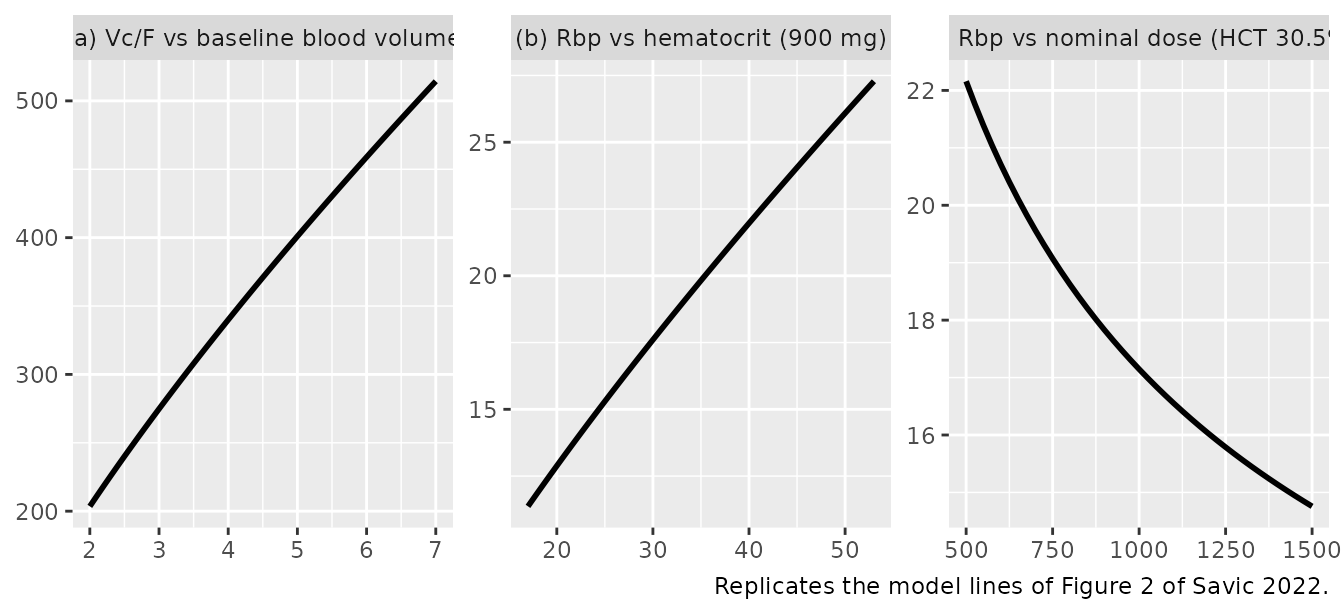
Virtual cohort
Original observed data are not publicly available. The steady-state comparison below uses two dose arms of 200 virtual adults each at the approved 1500 mg and the 900 mg dose, once daily. Covariates are drawn from log-normal distributions matched to the published summaries: blood volume median 3.9 L with the 10th-90th percentile range 2.9-5.2 L (Results), and hematocrit median 27% (the baseline median of Table 1) with the spread of the time-varying 10th-90th percentile range (24.3-37.7% around 30.5%). Nobody receives a CYP3A4 inducer (5% did in the source cohort).
set.seed(20220601)
rxode2::rxSetSeed(20220601)

n_per_arm <- 200
n_dose <- 42            # six weeks of once-daily dosing: past steady state
tau <- 24
t_last <- (n_dose - 1) * tau

make_cohort <- function(n, dose, id_offset) {
  tibble(
    id = id_offset + seq_len(n),
    treatment = paste(dose, "mg QD"),
    DOSE_VOXELOTOR_MG = dose,
    # 10th-90th percentile 2.9-5.2 L around 3.9 L: log-SD = log(5.2/2.9)/(2*1.2816)
    BLOOD_VOLUME = 3.9 * exp(rnorm(n, 0, log(5.2 / 2.9) / (2 * qnorm(0.9)))),
    # 10th-90th percentile 24.3-37.7% around 30.5%: same log-SD, centred on 27%
    HCT = 27 * exp(rnorm(n, 0, log(37.7 / 24.3) / (2 * qnorm(0.9)))),
    CONMED_CYP3A4_IND_WEAK = 0L,
    # Table 3 reports exposures from individual (between-subject) parameters,
    # so between-occasion variability is switched off with OCC = 0.
    OCC = 0L
  )
}

subjects <- dplyr::bind_rows(
  make_cohort(n_per_arm, 900, 0L),
  make_cohort(n_per_arm, 1500, n_per_arm)
)

doses <- subjects |>
  tidyr::crossing(time = seq(0, t_last, by = tau)) |>
  mutate(evid = 1L, amt = DOSE_VOXELOTOR_MG, cmt = "depot", dvid = NA_integer_)

obs <- subjects |>
  tidyr::crossing(time = c(seq(0, t_last - tau, by = tau),
                           t_last + c(0, 0.25, 0.5, 1, 1.5, 2, 3, 4, 5, 6, 8,
                                      10, 12, 16, 20, 24))) |>
  mutate(evid = 0L, amt = 0, cmt = "central", dvid = 1L)

events <- dplyr::bind_rows(doses, obs) |>
  arrange(id, time, desc(evid)) |>
  relocate(id, time, evid, amt, cmt, dvid)

stopifnot(!anyDuplicated(unique(events[, c("id", "time", "evid")])))
Simulation
sim <- rxode2::rxSolve(
  mod, events = events, keep = c("treatment"),
  returnType = "data.frame", useLinCmt = FALSE
)
# Steady-state profiles over the last dosing interval, plasma and whole blood.
sim |>
  filter(time >= t_last) |>
  select(id, time, treatment, Plasma = Cc, `Whole blood` = Cblood) |>
  tidyr::pivot_longer(c(Plasma, `Whole blood`), names_to = "matrix", values_to = "conc") |>
  group_by(time, treatment, matrix) |>
  summarise(Q05 = quantile(conc, 0.05), Q50 = median(conc),
            Q95 = quantile(conc, 0.95), .groups = "drop") |>
  ggplot(aes(time - t_last, Q50, colour = treatment, fill = treatment)) +
  geom_ribbon(aes(ymin = Q05, ymax = Q95), alpha = 0.2, colour = NA) +
  geom_line() +
  facet_wrap(~matrix, scales = "free_y") +
  labs(x = "Time after dose at steady state (h)", y = "Voxelotor (ug/mL)",
       colour = NULL, fill = NULL,
       caption = "Median and 90% interval of the virtual cohort.")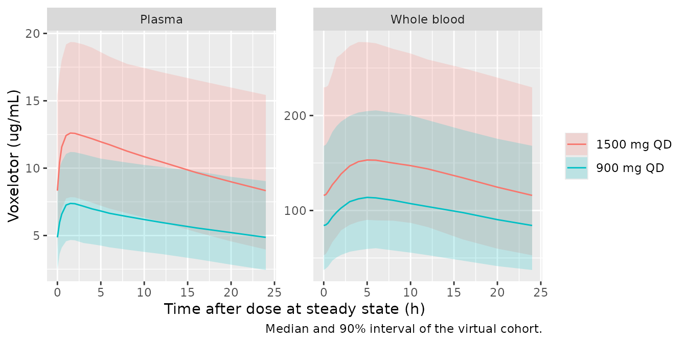
# Trough concentrations over the six weeks: steady state is reached within
# about three weeks (terminal half-life about 140 h for the typical patient).
sim |>
  filter(time > 0, time <= t_last, time %% tau == 0) |>
  group_by(time, treatment) |>
  summarise(Plasma = median(Cc), `Whole blood` = median(Cblood), .groups = "drop") |>
  tidyr::pivot_longer(c(Plasma, `Whole blood`), names_to = "matrix", values_to = "conc") |>
  ggplot(aes(time / 24, conc, colour = treatment)) +
  geom_line() + geom_point(size = 0.8) +
  facet_wrap(~matrix, scales = "free_y") +
  labs(x = "Day", y = "Median trough (ug/mL)", colour = NULL)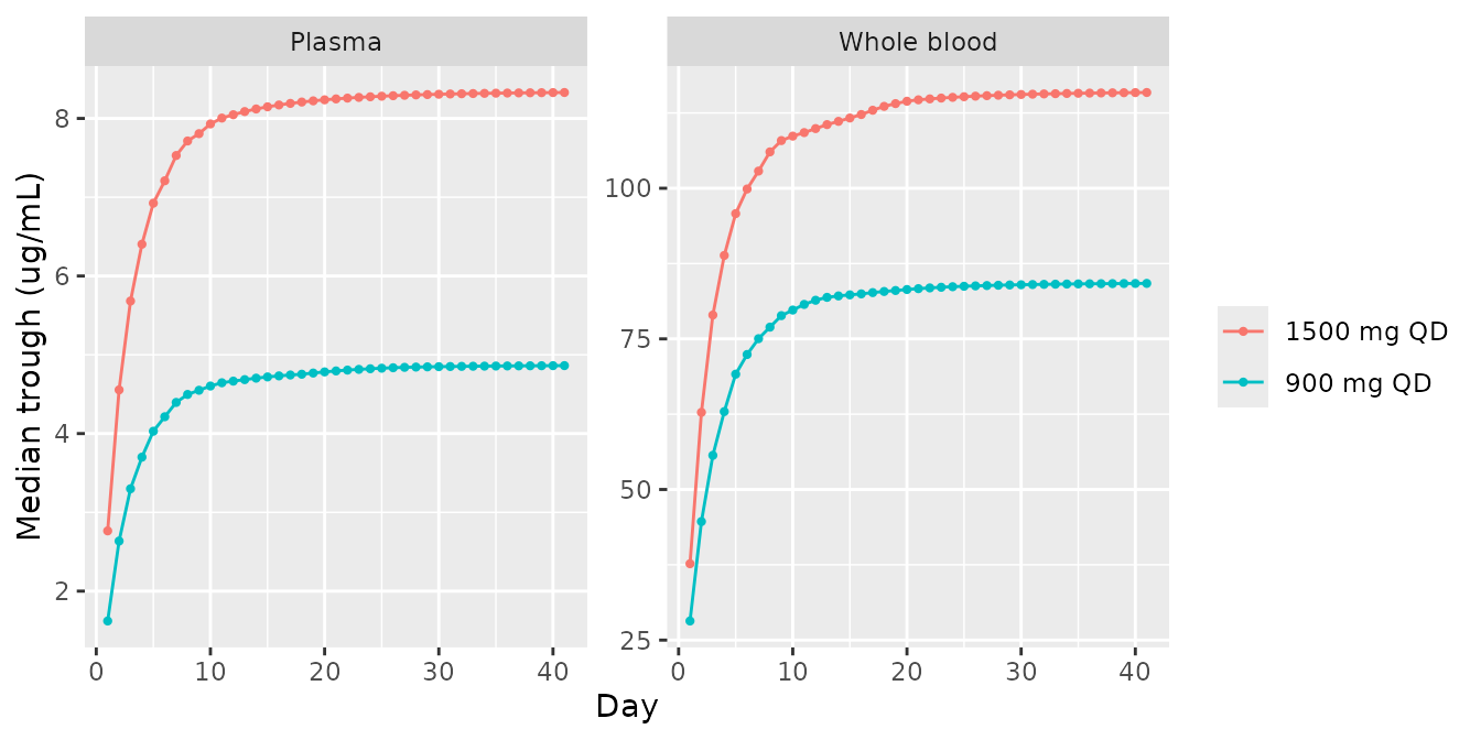
PKNCA validation
Steady-state NCA over the last 24-hour dosing interval, one PKNCA block per matrix, grouped by dose arm.
run_nca <- function(sim, conc_col) {
  conc <- sim |>
    filter(time >= t_last, !is.na(.data[[conc_col]])) |>
    transmute(id, treatment, time, conc = .data[[conc_col]])
  dose_df <- events |>
    filter(evid == 1, time == t_last) |>
    select(id, treatment, time, amt)
  conc_obj <- PKNCA::PKNCAconc(conc, conc ~ time | treatment + id)
  dose_obj <- PKNCA::PKNCAdose(dose_df, amt ~ time | treatment + id)
  intervals <- data.frame(start = t_last, end = t_last + tau,
                          cmax = TRUE, cmin = TRUE, tmax = TRUE, auclast = TRUE)
  PKNCA::pk.nca(PKNCA::PKNCAdata(conc_obj, dose_obj, intervals = intervals))
}

nca_plasma <- run_nca(sim, "Cc")
nca_blood <- run_nca(sim, "Cblood")
Comparison against Table 3
Table 3 of Savic 2022 reports geometric means of model-predicted steady-state exposures from the individual post hoc parameters; the adult columns (N = 70 at 900 mg, N = 68 at 1500 mg) are used. The simulated values are cohort medians, which for log-normal exposures estimate the geometric mean.
nca_units <- c(cmax = "ug/mL", cmin = "ug/mL", auclast = "h*ug/mL", tmax = "h")

ref_plasma <- tibble::tribble(
  ~treatment,    ~auclast, ~cmin, ~cmax,
  "900 mg QD",   142,      4.61,  7.24,
  "1500 mg QD",  274,      9.14,  13.7
)
ref_blood <- tibble::tribble(
  ~treatment,    ~auclast, ~cmin, ~cmax,
  "900 mg QD",   2250,     76.8,  107,
  "1500 mg QD",  3780,     132,   177
)

cmp_plasma <- nlmixr2lib::ncaComparisonTable(
  nca_plasma, ref_plasma, by = "treatment", units = nca_units,
  params = c("auclast", "cmin", "cmax")
)
cmp_blood <- nlmixr2lib::ncaComparisonTable(
  nca_blood, ref_blood, by = "treatment", units = nca_units,
  params = c("auclast", "cmin", "cmax")
)
cmp <- dplyr::bind_rows(
  cmp_plasma |> mutate(Matrix = "Plasma", .before = 1),
  cmp_blood |> mutate(Matrix = "Whole blood", .before = 1)
)
knitr::kable(cmp, caption = "Simulated (median) vs Table 3 (adult geometric mean). * differs by more than 20%.")| Matrix | NCA parameter | treatment | Reference | Simulated | % diff |
|---|---|---|---|---|---|
| Plasma | Cmax (ug/mL) | 900 mg QD | 7.24 | 7.38 | +1.9% |
| Plasma | Cmax (ug/mL) | 1500 mg QD | 13.7 | 12.6 | -8.0% |
| Plasma | Cmin (ug/mL) | 900 mg QD | 4.61 | 4.86 | +5.5% |
| Plasma | Cmin (ug/mL) | 1500 mg QD | 9.14 | 8.33 | -8.9% |
| Plasma | AUClast (h*ug/mL) | 900 mg QD | 142 | 143 | +1.0% |
| Plasma | AUClast (h*ug/mL) | 1500 mg QD | 274 | 251 | -8.4% |
| Whole blood | Cmax (ug/mL) | 900 mg QD | 107 | 114 | +6.6% |
| Whole blood | Cmax (ug/mL) | 1500 mg QD | 177 | 153 | -13.4% |
| Whole blood | Cmin (ug/mL) | 900 mg QD | 76.8 | 84.2 | +9.7% |
| Whole blood | Cmin (ug/mL) | 1500 mg QD | 132 | 116 | -12.2% |
| Whole blood | AUClast (h*ug/mL) | 900 mg QD | 2250 | 2410 | +6.9% |
| Whole blood | AUClast (h*ug/mL) | 1500 mg QD | 3780 | 3310 | -12.3% |
nca_med <- dplyr::bind_rows(
  as.data.frame(nca_plasma$result) |> mutate(matrix = "plasma"),
  as.data.frame(nca_blood$result) |> mutate(matrix = "blood")
) |>
  filter(PPTESTCD %in% c("auclast", "cmin", "cmax")) |>
  group_by(matrix, treatment, PPTESTCD) |>
  summarise(sim = median(PPORRES), .groups = "drop")

ref_long <- dplyr::bind_rows(
  ref_plasma |> mutate(matrix = "plasma"),
  ref_blood |> mutate(matrix = "blood")
) |>
  tidyr::pivot_longer(c(auclast, cmin, cmax), names_to = "PPTESTCD", values_to = "ref")

gate <- inner_join(nca_med, ref_long, by = c("matrix", "treatment", "PPTESTCD")) |>
  mutate(pct_diff = 100 * (sim - ref) / ref)
stopifnot(nrow(gate) == 12)

# Centre of the distribution, not its tails: a mis-transcribed clearance,
# volume, ratio or unit moves these medians by tens of percent or by orders
# of magnitude. The 25% bound holds the differences discussed below
# (largest about 13%) with room for cohort-to-cohort noise in a 200-subject
# median (about 2-3%).
stopifnot(all(abs(gate$pct_diff) < 25))
Every simulated exposure is within 20% of Table 3: the 900 mg arm sits 1-10% above the paper and the 1500 mg arm 8-13% below it. The split comes from the paper’s own numbers. The model is linear in dose, so its 1500:900 plasma AUC ratio is the dose ratio, 1.67. Table 3’s adult ratio is 274 / 142 = 1.93, because its geometric means come from the post hoc estimates of the patients actually treated at each dose: the 1500 mg adults imply an apparent clearance of 1500 / 274 = 5.5 L/h and the 900 mg adults 900 / 142 = 6.3 L/h, either side of the typical 6.14 L/h of Table 2. Whole blood at 1500 mg is a few percent further below the paper than plasma because hematocrit rose more on the higher dose (geometric-mean maximum 35.1% against 32.6%, Table S4) while the virtual cohort holds both arms at the same hematocrit.
Whole-blood-to-plasma partitioning and Hb occupancy
Over a steady-state dosing interval the effect compartment carries
the same area as plasma, so the whole-blood-to-plasma AUC ratio equals
each subject’s Rbp. Percent Hb occupancy follows the
paper’s definition, the red-cell voxelotor concentration over the 5000
uM red-cell Hb concentration, with the red-cell concentration
(C_WB - (1 - HCT) * C_plasma) / HCT. Converting ug/mL to uM
needs the molecular weight of voxelotor, 337.37 g/mol (PubChem CID
71602803), which the paper does not print.
mw <- 337.37   # g/mol, voxelotor (PubChem); not stated in Savic 2022

hct_by_id <- subjects |> select(id, HCT)

occ <- dplyr::bind_rows(
  as.data.frame(nca_plasma$result) |> mutate(matrix = "plasma"),
  as.data.frame(nca_blood$result) |> mutate(matrix = "blood")
) |>
  filter(PPTESTCD %in% c("cmin", "cmax", "auclast")) |>
  select(id, treatment, matrix, PPTESTCD, PPORRES) |>
  tidyr::pivot_wider(names_from = c(matrix, PPTESTCD), values_from = PPORRES) |>
  left_join(hct_by_id, by = "id") |>
  mutate(
    hct = HCT / 100,
    ratio_auc = blood_auclast / plasma_auclast,
    occ_cmin = 100 * ((blood_cmin - (1 - hct) * plasma_cmin) / hct) / mw * 1000 / 5000,
    occ_cmax = 100 * ((blood_cmax - (1 - hct) * plasma_cmax) / hct) / mw * 1000 / 5000
  )

occ_summary <- occ |>
  group_by(treatment) |>
  summarise(
    `WB:plasma AUC ratio` = median(ratio_auc),
    `% Hb occupancy at Cmin` = median(occ_cmin),
    `% Hb occupancy at Cmax` = median(occ_cmax),
    .groups = "drop"
  ) |>
  left_join(
    tibble::tribble(
      ~treatment,   ~`Table 3 ratio (AUC WB / AUC plasma)`, ~`Table 3 occupancy at Cmin`, ~`Table 3 occupancy at Cmax`,
      "900 mg QD",  2250 / 142,                             16.2,                         22.4,
      "1500 mg QD", 3780 / 274,                             26.5,                         35.4
    ),
    by = "treatment"
  )
knitr::kable(occ_summary, digits = 1,
caption = "Simulated medians against the Table 3 adult geometric means.")| treatment | WB:plasma AUC ratio | % Hb occupancy at Cmin | % Hb occupancy at Cmax | Table 3 ratio (AUC WB / AUC plasma) | Table 3 occupancy at Cmin | Table 3 occupancy at Cmax |
|---|---|---|---|---|---|---|
| 1500 mg QD | 13.9 | 24.5 | 31.3 | 13.8 | 26.5 | 35.4 |
| 900 mg QD | 16.6 | 17.6 | 23.5 | 15.8 | 16.2 | 22.4 |
stopifnot(
  abs(occ_summary$`% Hb occupancy at Cmin` / occ_summary$`Table 3 occupancy at Cmin` - 1) < 0.25,
  abs(occ_summary$`% Hb occupancy at Cmax` / occ_summary$`Table 3 occupancy at Cmax` - 1) < 0.25
)
The simulated occupancy at trough is about 18% at 900 mg and 25% at 1500 mg, against 16.2% and 26.5% in Table 3, and at the peak about 24% and 31% against 22.4% and 35.4%. The arms differ from the paper in the same directions as the exposures above. The simulated whole-blood-to-plasma AUC ratios (about 16.6 and 13.9) are within 5% of the ratios implied by Table 3 (15.8 and 13.8).
Plasma half-life
Table 3 lists a plasma half-life of 35.6 h (900 mg) and 39.4 h (1500
mg) in adults. That matches the first (dominant) disposition phase of
the two-compartment model, log(2) / lambda1, not the slow
terminal phase; for the typical patient the two are about 35 h and 140
h. The simulated geometric means (about 34 h in both arms) are 4% and
13% below Table 3; the model’s half-life does not depend on dose, while
the 1500 mg patients of Table 3 had the lower post hoc clearances
discussed above.
hl <- sim |>
  filter(time == t_last) |>
  distinct(id, treatment, cl, vc, q, vp) |>
  mutate(
    k10 = cl / vc, k12 = q / vc, k21 = q / vp,
    s = k10 + k12 + k21,
    lambda1 = (s + sqrt(s^2 - 4 * k10 * k21)) / 2,
    lambda2 = (s - sqrt(s^2 - 4 * k10 * k21)) / 2,
    t_half_1 = log(2) / lambda1,
    t_half_terminal = log(2) / lambda2
  )
hl_summary <- hl |>
  group_by(treatment) |>
  summarise(`Dominant-phase t1/2 (h)` = exp(mean(log(t_half_1))),
            `Terminal t1/2 (h)` = exp(mean(log(t_half_terminal))),
            .groups = "drop") |>
  mutate(`Table 3 t1/2 (h)` = c(`1500 mg QD` = 39.4, `900 mg QD` = 35.6)[treatment])
knitr::kable(hl_summary, digits = 1,
caption = "Geometric-mean half-lives from the individual parameters.")| treatment | Dominant-phase t1/2 (h) | Terminal t1/2 (h) | Table 3 t1/2 (h) |
|---|---|---|---|
| 1500 mg QD | 34.4 | 141.4 | 39.4 |
| 900 mg QD | 34.0 | 141.2 | 35.6 |
Assumptions and deviations
-
Structure of the whole-blood link. The paper
describes the link only in words and in Figure 1 (an effect compartment
with
KbpandRbpon the plasma-to-whole-blood arrow). The model uses the standard effect-compartment form,d/dt(effect) = Kbp * (Cc - effect)withCblood = Rbp * effect. WritingRbpinside the derivative instead (d/dt(Cblood) = Kbp * (Rbp * Cc - Cblood)) gives identical predictions wheneverRbpis constant, and differs only transiently, over a few hours (1 /Kbp= 2.3 h), when time-varying hematocrit changes, which happens over weeks. - No BSV on Ka. The Results say the original plasma model “was updated to also include BSV on … Ka”, but the final-model Table 2 fixes Ka at 2.38 1/h and lists no BSV on it, so the model carries none.
-
Between-occasion variability. BOV on CL/F (56.3%
CV) is encoded as 13 occasion etas sharing one variance, selected by the
OCCcolumn (1-13). The paper does not print which sampling visit maps to which occasion. SettingOCC = 0(any value outside 1-13) switches BOV off; the steady-state comparison does this because Table 3 comes from between-subject individual parameters. - Whole-blood residual error. Table 2 gives an additive and a proportional term for whole blood without saying how they combine; the model uses nlmixr2’s default combined form (variances add). The additive 880 ng/mL is converted to 0.88 ug/mL to match the model’s concentration units.
-
Blood volume. The paper says blood volume was
“calculated based on body weight and sex” but does not give the formula,
so
BLOOD_VOLUMEis a user-supplied column. The virtual cohort draws it directly from the published percentiles rather than from body weight. -
Nominal dose.
DOSE_VOXELOTOR_MGis the nominal dose of the regimen (500-1500 mg). The paper does not say how the 500 mg twice-daily arm of the first-in-human study was coded. -
Hematocrit in the virtual cohort. The steady-state
cohort is centred on the baseline median hematocrit of 27%. Hematocrit
rises on treatment (median 30.5% over time), which would raise
Rbpand whole-blood exposure by about 10% ((30.5 / 27)^0.77 = 1.10). The whole-blood-to-plasma AUC ratios implied by Table 3 (15.8 at 900 mg, 13.8 at 1500 mg) correspond to the model’sRbpat a hematocrit of about 26% and 28%, consistent with that choice. - Molecular weight. The 337.37 g/mol used for Hb occupancy is from PubChem; the paper does not state it.
- CYP3A4 inducers. The coefficient applies to weak inducers only, the only class present in the data (14 of 264 PK-evaluable patients); strong inducers were prohibited.
- Errata. No correction notice for this article was found on the Crossref record (no update-to or updated-by entries) or in Europe PMC as of 2026-10-01.