Alemtuzumab (Admiraal 2019)

Model and source

• Citation: Admiraal R, Jol-van der Zijde CM, Furtado Silva JM, Knibbe CAJ, Lankester AC, Boelens JJ, Hale G, Etuk A, Wilson M, Adams S, Veys P, van Kesteren C, Bredius RGM. Population Pharmacokinetics of Alemtuzumab (Campath) in Pediatric Hematopoietic Cell Transplantation: Towards Individualized Dosing to Improve Outcome. Clin Pharmacokinet. 2019;58(12):1609-1620. doi:10.1007/s40262-019-00782-0
• Description: Two-compartment population PK model with parallel linear and Michaelis-Menten elimination for intravenous alemtuzumab in children undergoing allogeneic hematopoietic cell transplantation, with a body-weight-dependent exponent on linear clearance (Admiraal 2019)
• Article: Clin Pharmacokinet 2019;58:1609-1620 (open access, PMC6885503). The electronic supplementary material contains the full NONMEM control stream of the final model.

Admiraal et al. described the pharmacokinetics of alemtuzumab (Campath), an anti-CD52 monoclonal antibody given as serotherapy in the conditioning regimen of paediatric allogeneic haematopoietic cell transplantation (HCT). The final model is two-compartmental with parallel linear and Michaelis-Menten elimination from the central compartment. Body weight scales the central volume (V1) and the intercompartmental clearance (Q) as fixed power functions, and the linear clearance (CL) through a body-weight-dependent exponent (BDE) whose value itself falls with weight:

$$CL_i = CL_{pop} \cdot \left(\frac{WT}{17.25}\right)^{(a \cdot WT)^b} \cdot e^{\eta_{CL}}$$

The peripheral volume is estimated as a factor of the individual central volume (V2 = 0.7 x V1). Baseline lymphocyte count was tested and did not affect any parameter.

Population

The model was developed from 1146 alemtuzumab concentrations in 206 children (212 HCTs) treated at Leiden University Medical Center (67 patients, 73 HCTs) and Great Ormond Street Hospital, London (139 patients) between 2003 and 2015 (Admiraal 2019 Table 1). Median age was 4.8 years (range 0.2-19; 28 infants younger than 1 year), median weight 17.2 kg (IQR 11-32), and 67% were male. The most common indication was immune deficiency (52%), followed by haematologic malignancy (25%) and bone marrow failure (18%). Alemtuzumab was infused intravenously, usually as 0.2 mg/kg/day on 4-5 consecutive days starting a median of 8 days before graft infusion; 54% of patients received a cumulative 0.9-1.1 mg/kg and 35% less than 0.9 mg/kg. Race was not reported.

The same information is available programmatically via readModelDb("Admiraal_2019_alemtuzumab")()$population.

Source trace

Every value below is also recorded as an in-file comment next to the matching ini() entry in inst/modeldb/specificDrugs/Admiraal_2019_alemtuzumab.R. ESM denotes the NONMEM control stream (run28) in the electronic supplementary material.

Equation / parameter	Value	Source location
Two-compartment, IV, parallel linear + Michaelis-Menten CL from central	n/a	Results 3.2; ESM $DES
lcl (linear CL at 17.25 kg)	log(0.25 L/day)	Table 2 CL pop; ESM THETA(1)
e_wt_cl_bdecoef (a)	0.038 1/kg	Table 2 a; ESM THETA(7)
e_wt_cl_bdeexp (b)	-0.79	Table 2 b; ESM THETA(8)
BDE form (WT/17.25)^((a*WT)^b)	n/a	Methods Eq. 7; Table 2; ESM TVCL = THETA(1) * (MWT**((THETA(7)*WT)**THETA(8)))
lvc (V1 at 17.25 kg)	log(2.13 L)	Table 2 V1,pop; ESM THETA(2)
e_wt_vc (c)	0.58	Table 2 c; ESM THETA(9)
lvp_ratio (V2 / V1)	log(0.7)	Table 2 V2,pop (factor of V1); ESM V2 = V1 * THETA(3)
lq (Q at 17.25 kg)	log(0.18 L/day)	Table 2 Q; ESM THETA(4)
e_wt_q (d)	0.74	Table 2 d; ESM THETA(10)
lvmax	log(0.42 mg/day)	Table 2 Vmax,pop (AU/day); ESM THETA(5)
lkm	log(1.38 mg/L)	Table 2 Km,pop (AU/L); ESM THETA(6)
Reference weight	17.25 kg	ESM MWT = WT/17.25
etalcl	0.73314 (104% CV)	Table 2 IIV on CL
etalvc	0.33426 (63% CV)	Table 2 IIV on V1
etalkm	1.06623 (138% CV)	Table 2 IIV on Km
No IIV on Q, V2 (other than through V1) or Vmax	n/a	ESM $PK (Q = TVQ, VMAX = TVVMAX)
expSd	0.34	Table 2 Proportional residual error (%) = 34; ESM $ERROR Y = IPRED + ERR(1) on log-transformed data

Body-weight-dependent exponent on linear clearance

The paper reports that the exponent “varied from 3.69 in children with a body weight of 5 kg to 0.41 in patients weighing 80 kg” (Results 3.3, electronic supplementary Fig. S3), and that linear CL “is expected to slightly decrease from a body weight of 60 kg onwards (decrease of 1.2%)” (Discussion). Both follow deterministically from the packaged ini() values.

mod <- readModelDb("Admiraal_2019_alemtuzumab")
ini_vals <- rxode2::rxode(mod)$theta
#> ℹ parameter labels from comments will be replaced by 'label()'

bde <- tibble(WT = seq(3, 90, by = 0.5)) |>
  mutate(
    exponent = (ini_vals[["e_wt_cl_bdecoef"]] * WT)^ini_vals[["e_wt_cl_bdeexp"]],
    cl_linear = exp(ini_vals[["lcl"]]) * (WT / 17.25)^exponent
  )

exponent_at <- function(wt) {
  (ini_vals[["e_wt_cl_bdecoef"]] * wt)^ini_vals[["e_wt_cl_bdeexp"]]
}
cl_at <- function(wt) exp(ini_vals[["lcl"]]) * (wt / 17.25)^exponent_at(wt)

bde_check <- tibble(
  Quantity = c(
    "Exponent at 5 kg",
    "Exponent at 80 kg",
    "Change in linear CL, 60 to 80 kg (%)"
  ),
  Published = c(3.69, 0.41, -1.2),
  Model = c(exponent_at(5), exponent_at(80), 100 * (cl_at(80) / cl_at(60) - 1))
)
knitr::kable(bde_check, digits = 3)

Quantity	Published	Model
Exponent at 5 kg	3.69	3.714
Exponent at 80 kg	0.41	0.415
Change in linear CL, 60 to 80 kg (%)	-1.20	-1.255

# The published figures were computed from unrounded estimates; a and b are
# printed to two significant figures, so agreement is to that rounding only.
stopifnot(
  abs(bde_check$Model[1] / 3.69 - 1) < 0.02,
  abs(bde_check$Model[2] / 0.41 - 1) < 0.03,
  round(bde_check$Model[3], 1) %in% c(-1.2, -1.3)
)

bde |>
  pivot_longer(c(exponent, cl_linear), names_to = "quantity") |>
  mutate(
    quantity = factor(
      quantity,
      levels = c("exponent", "cl_linear"),
      labels = c("A: scaling exponent (a x WT)^b", "B: typical linear CL (L/day)")
    )
  ) |>
  ggplot(aes(WT, value)) +
  geom_line() +
  facet_wrap(~quantity, scales = "free_y") +
  labs(x = "Body weight (kg)", y = NULL) +
  theme_bw()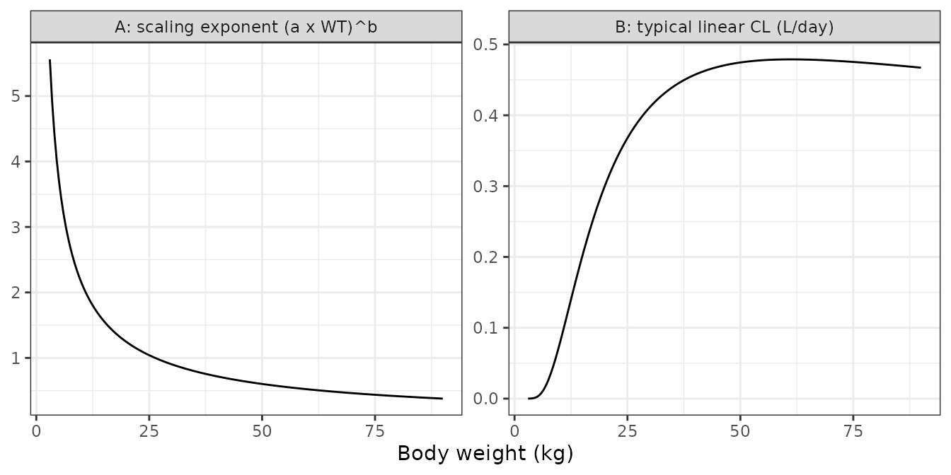

Replicates electronic supplementary Fig. S3 of Admiraal 2019: (A) the BDE scaling exponent on linear CL and (B) typical linear CL, both against body weight.

Contribution of linear and saturable clearance

Total clearance at concentration C is the linear CL plus the instantaneous Michaelis-Menten clearance V_max / (K_m + C). The figure reproduces electronic supplementary Fig. S2 for the 17.25 kg reference child.

cl_conc <- tibble(conc = 10^seq(-2, 1.3, length.out = 200)) |>
  mutate(
    Linear = exp(ini_vals[["lcl"]]),
    Saturable = exp(ini_vals[["lvmax"]]) / (exp(ini_vals[["lkm"]]) + conc),
    Total = Linear + Saturable
  ) |>
  pivot_longer(-conc, names_to = "pathway", values_to = "cl")

ggplot(cl_conc, aes(conc, cl, linetype = pathway)) +
  geom_line() +
  scale_x_log10() +
  scale_linetype_manual(values = c(Linear = "dotdash", Saturable = "dashed", Total = "solid")) +
  labs(x = "Alemtuzumab concentration (mg/L)", y = "Clearance (L/day)", linetype = NULL) +
  theme_bw()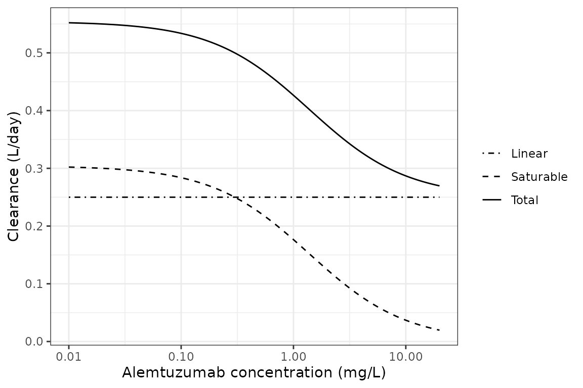

Replicates electronic supplementary Fig. S2 of Admiraal 2019: typical total, linear and saturable clearance against serum alemtuzumab concentration (17.25 kg child).

# At concentrations far below Km the saturable pathway approaches Vmax/Km.
stopifnot(abs(
  exp(ini_vals[["lvmax"]]) / (exp(ini_vals[["lkm"]]) + 1e-6) -
    exp(ini_vals[["lvmax"]] - ini_vals[["lkm"]])
) < 1e-6)

Virtual cohort

Observed data are not public. The virtual cohort draws body weight from a log-normal distribution with the published median (17.2 kg) and a spread that reproduces the published interquartile range (11-32 kg), truncated to 3-90 kg. Every subject receives the most common regimen, 0.2 mg/kg/day on five consecutive days (cumulative 1 mg/kg), with day 0 the first infusion as in Fig. 1 of the paper. Infusion duration is not reported; 4 hours is assumed.

set.seed(2019)
n_sub <- 200
wt_sdlog <- (log(32) - log(11)) / (2 * qnorm(0.75))

cohort <- tibble(
  id = seq_len(n_sub),
  WT = pmin(pmax(rlnorm(n_sub, log(17.2), wt_sdlog), 3), 90)
) |>
  mutate(
    wt_band = cut(
      WT,
      breaks = c(0, 11, 17.3, 32, Inf),
      labels = c("<11 kg", "11-17.3 kg", "17.3-32 kg", ">32 kg"),
      right = FALSE
    )
  )

dose_days <- 0:4
# Includes the bin times digitised from Fig. 4e below.
obs_times <- sort(unique(c(
  seq(0, 6, by = 0.125),
  seq(6.5, 14, by = 0.5),
  seq(15, 80, by = 1),
  c(21.5, 28.5, 53.5)
)))

dose_rows <- cohort |>
  tidyr::crossing(time = dose_days) |>
  mutate(evid = 1L, amt = 0.2 * WT, dur = 4 / 24, cmt = "central")
obs_rows <- cohort |>
  tidyr::crossing(time = obs_times) |>
  mutate(evid = 0L, amt = 0, dur = 0, cmt = "central")
events <- bind_rows(dose_rows, obs_rows) |>
  arrange(id, time, desc(evid)) |>
  as.data.frame()

table(cohort$wt_band)
#> 
#>     <11 kg 11-17.3 kg 17.3-32 kg     >32 kg 
#>         60         56         49         35

Simulation

rxode2::rxSetSeed(2019)
sim <- rxode2::rxSolve(
  mod,
  events = events,
  keep = c("WT", "wt_band"),
  returnType = "data.frame"
)
#> ℹ parameter labels from comments will be replaced by 'label()'
# Concentrations at the observation records only (evid is not returned).
sim <- sim |> filter(!is.na(Cc))

# Population predictions (no between-subject or residual variability) for
# the prediction correction below.
pred <- rxode2::rxSolve(
  rxode2::zeroRe(mod),
  events = events,
  returnType = "data.frame"
) |>
  filter(!is.na(Cc)) |>
  select(id, time, pred = Cc)
#> ℹ parameter labels from comments will be replaced by 'label()'
#> ℹ omega/sigma items treated as zero: 'etalcl', 'etalvc', 'etalkm'
#> Warning: multi-subject simulation without without 'omega'

Prediction-corrected VPC (Figure 4e)

Fig. 4e of the paper is a prediction-corrected VPC on a log axis. Its simulated median falls about 3-fold between days 15 and 50, far less than the terminal half-life of the typical patient (about 8 days at low concentrations) allows. The flattening appears once simulated values below the 0.1 ug/mL limit of quantification are removed before the percentiles are taken, which is the usual way a VPC with an LLOQ is built. Only the subjects whose concentrations remain measurable then contribute late in the profile. The chunk below repeats the prediction correction (each simulated value scaled by the bin median of the population prediction over the subject’s own population prediction) with and without that censoring. It overlays the simulated percentiles digitised from Fig. 4e (dotted lines in the paper; read from the raster at about +/-10%).

lloq <- 0.1

pc_percentiles <- function(d) {
  d |>
    group_by(time) |>
    mutate(pc = sim * median(pred) / pred) |>
    summarise(
      p05 = quantile(pc, 0.05),
      p50 = quantile(pc, 0.50),
      p95 = quantile(pc, 0.95),
      .groups = "drop"
    )
}

sim_pred <- sim |>
  select(id, time, sim) |>
  left_join(pred, by = c("id", "time")) |>
  filter(time > 0)

vpc <- bind_rows(
  sim_pred |> filter(sim >= lloq) |> pc_percentiles() |> mutate(censoring = "Below LLOQ removed"),
  sim_pred |> pc_percentiles() |> mutate(censoring = "All simulated values")
)

# Simulated (dotted) percentiles of Fig. 4e, read from the published figure.
fig4e <- tibble(
  time = c(4.5, 10.5, 15, 21.5, 28.5, 36, 47, 53.5),
  p05 = c(0.98, 0.143, 0.103, 0.086, 0.052, 0.065, 0.033, 0.034),
  p50 = c(4.0, 1.46, 0.96, 0.65, 0.54, 0.42, 0.31, 0.32),
  p95 = c(13.4, 6.4, 5.1, 3.6, 3.3, 2.96, 2.45, 2.45)
)

vpc_long <- vpc |>
  pivot_longer(c(p05, p50, p95), names_to = "percentile")
fig4e_long <- fig4e |>
  pivot_longer(c(p05, p50, p95), names_to = "percentile")

ggplot(vpc_long, aes(time, value, group = interaction(percentile, censoring))) +
  geom_line(aes(linetype = censoring)) +
  geom_point(data = fig4e_long, aes(group = percentile, shape = percentile)) +
  scale_y_log10() +
  scale_linetype_manual(values = c("Below LLOQ removed" = "solid", "All simulated values" = "dashed")) +
  coord_cartesian(xlim = c(0, 60), ylim = c(1e-2, 30)) +
  labs(
    x = "Time since first alemtuzumab dose (days)",
    y = "Prediction-corrected alemtuzumab (mg/L)",
    linetype = NULL,
    shape = "Fig. 4e"
  ) +
  theme_bw()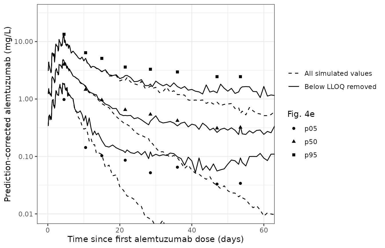

Replicates the simulated percentiles of Fig. 4e of Admiraal 2019 (prediction-corrected VPC). Lines: 5th, 50th and 95th percentiles of the simulated concentrations including residual error, after removing simulated values below the 0.1 ug/mL LLOQ (solid) or keeping them (dashed). Points: the paper’s simulated percentiles, digitised.

vpc_cmp <- vpc |>
  filter(censoring == "Below LLOQ removed") |>
  inner_join(fig4e, by = "time", suffix = c("_sim", "_paper")) |>
  mutate(ratio_p50 = p50_sim / p50_paper)

vpc_cmp |>
  select(time, p50_sim, p50_paper, ratio_p50, p95_sim, p95_paper) |>
  dplyr::rename(
    "Day" = time,
    "Median, simulated" = p50_sim,
    "Median, Fig. 4e" = p50_paper,
    "Ratio" = ratio_p50,
    "95th pct, simulated" = p95_sim,
    "95th pct, Fig. 4e" = p95_paper
  ) |>
  knitr::kable(digits = 2)

Day	Median, simulated	Median, Fig. 4e	Ratio	95th pct, simulated	95th pct, Fig. 4e
4.5	4.60	4.00	1.15	12.92	13.40
10.5	1.68	1.46	1.15	5.11	6.40
15.0	0.94	0.96	0.98	3.01	5.10
21.5	0.52	0.65	0.80	2.56	3.60
28.5	0.41	0.54	0.76	1.82	3.30
36.0	0.34	0.42	0.81	1.65	2.96
47.0	0.26	0.31	0.85	1.28	2.45
53.5	0.34	0.32	1.06	1.54	2.45

late_uncensored <- vpc |>
  filter(censoring == "All simulated values", time %in% c(47, 53.5))
late_censored <- vpc |>
  filter(censoring == "Below LLOQ removed", time %in% c(47, 53.5))

stopifnot(
  # Centre: the censored median tracks the paper's simulated median over the
  # whole profile (typical ratio within 35%), which a wrong clearance, volume
  # or Michaelis-Menten constant would not.
  abs(log(median(vpc_cmp$ratio_p50))) < log(1.35),
  # The late flattening in Fig. 4e comes from the censoring: without it the
  # late median is several-fold lower.
  all(late_censored$p50 > 3 * late_uncensored$p50)
)

The typical-value profiles below show the non-linear influence of weight under uniform mg/kg dosing that motivates the paper’s conclusion: larger children reach higher peaks because V1 rises less than proportionally with weight (exponent 0.58), while in the smallest children the linear pathway is almost absent and elimination is dominated by the saturable pathway.

typical_wt <- c(5, 11, 17.25, 32, 60)
typical_events <- tibble(id = seq_along(typical_wt), WT = typical_wt) |>
  tidyr::crossing(time = dose_days) |>
  mutate(evid = 1L, amt = 0.2 * WT, dur = 4 / 24, cmt = "central") |>
  bind_rows(
    tibble(id = seq_along(typical_wt), WT = typical_wt) |>
      tidyr::crossing(time = obs_times) |>
      mutate(evid = 0L, amt = 0, dur = 0, cmt = "central")
  ) |>
  arrange(id, time, desc(evid)) |>
  as.data.frame()

typical <- rxode2::rxSolve(
  rxode2::zeroRe(mod),
  events = typical_events,
  keep = "WT",
  returnType = "data.frame"
) |>
  filter(!is.na(Cc))
#> ℹ parameter labels from comments will be replaced by 'label()'
#> ℹ omega/sigma items treated as zero: 'etalcl', 'etalvc', 'etalkm'
#> Warning: multi-subject simulation without without 'omega'

ggplot(typical, aes(time, Cc, colour = factor(WT))) +
  geom_line() +
  scale_y_log10() +
  coord_cartesian(ylim = c(1e-2, 20)) +
  labs(
    x = "Time since first alemtuzumab dose (days)",
    y = "Alemtuzumab (mg/L)",
    colour = "Weight (kg)"
  ) +
  theme_bw()
#> Warning in scale_y_log10(): log-10 transformation introduced infinite values.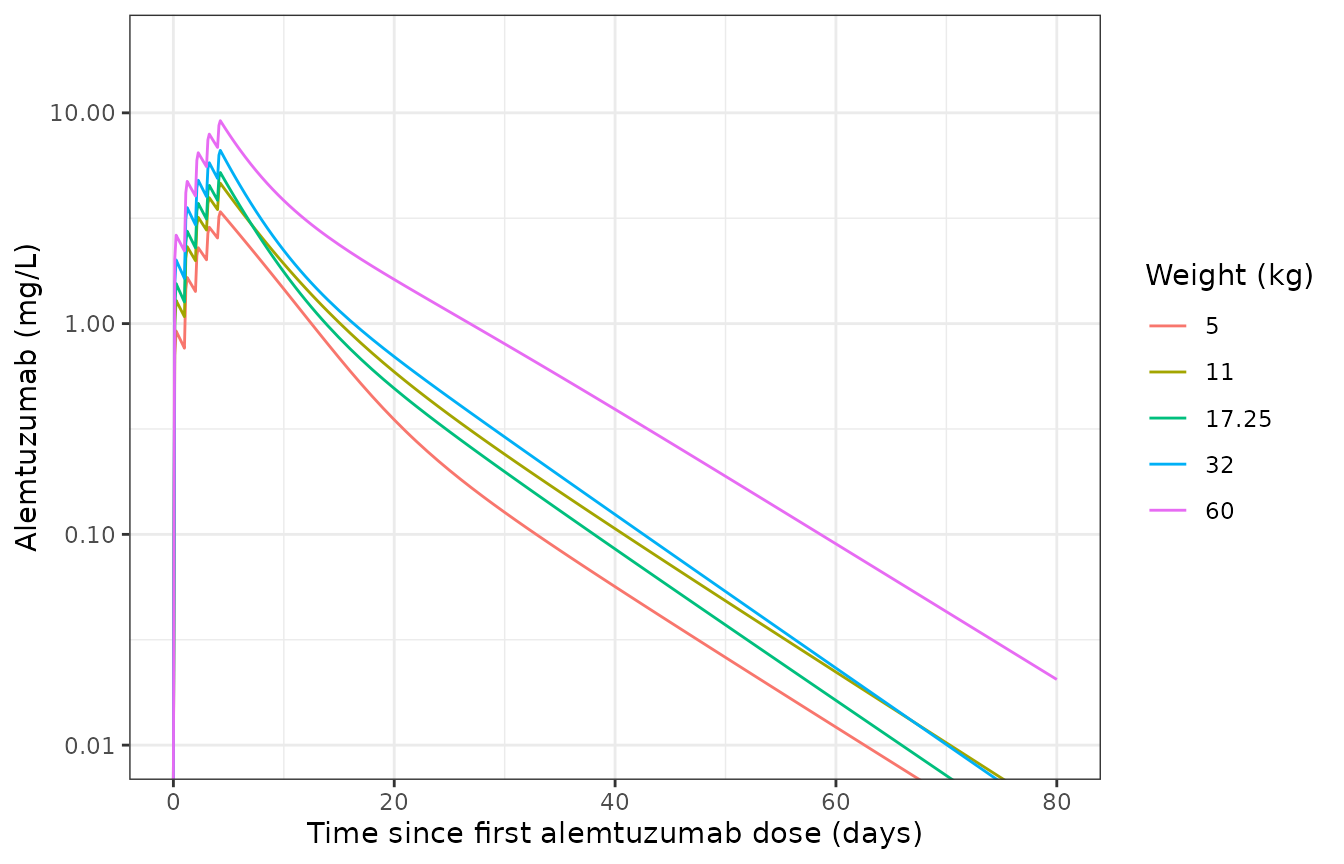

Typical concentration-time profiles (no between-subject variability) for children of 5, 11, 17.25, 32 and 60 kg receiving 0.2 mg/kg/day for 5 days.

PKNCA validation

NCA is run per subject over the full 80-day profile with weight quartile band (the bands of Fig. 2 of the paper) as the grouping variable.

# Integrator noise can leave a tail value a hair below zero; assert it is noise,
# floor it, and drop the numerically-zero tail so the half-life fit does not
# follow it (rising-phase points are kept).
stopifnot(all(sim$Cc >= -1e-6 * max(sim$Cc), na.rm = TRUE))
conc_df <- sim |>
  mutate(Cc = pmax(Cc, 0)) |>
  group_by(id) |>
  filter(time <= time[which.max(Cc)] | Cc >= 1e-6 * max(Cc)) |>
  ungroup() |>
  select(id, time, Cc, wt_band)

dose_df <- dose_rows |>
  select(id, time, amt, wt_band)

conc_obj <- PKNCA::PKNCAconc(conc_df, Cc ~ time | wt_band + id)
dose_obj <- PKNCA::PKNCAdose(dose_df, amt ~ time | wt_band + id)
intervals <- data.frame(
  start = 0,
  end = 80,
  cmax = TRUE,
  tmax = TRUE,
  auclast = TRUE,
  half.life = TRUE
)
nca <- PKNCA::pk.nca(PKNCA::PKNCAdata(conc_obj, dose_obj, intervals = intervals))

nca_summary <- as.data.frame(nca$result) |>
  filter(PPTESTCD %in% c("cmax", "tmax", "auclast", "half.life")) |>
  group_by(wt_band, PPTESTCD) |>
  summarise(median = median(PPORRES, na.rm = TRUE), .groups = "drop") |>
  pivot_wider(names_from = PPTESTCD, values_from = median)

nca_summary |>
  dplyr::rename(
    "Weight band" = wt_band,
    "Cmax (mg/L)" = cmax,
    "Tmax (day)" = tmax,
    "AUC0-80 (mg*day/L)" = auclast,
    "t1/2 (day)" = half.life
  ) |>
  knitr::kable(digits = 2, caption = "Median simulated NCA parameters by weight band, 0.2 mg/kg/day for 5 days.")

Median simulated NCA parameters by weight band, 0.2 mg/kg/day for 5 days.

Weight band	AUC0-80 (mg*day/L)	Cmax (mg/L)	t1/2 (day)	Tmax (day)
<11 kg	36.88	3.66	8.75	4.25
11-17.3 kg	43.38	4.98	8.23	4.25
17.3-32 kg	46.42	4.52	9.84	4.25
>32 kg	76.62	8.23	8.44	4.25

The paper does not tabulate NCA parameters, so there is no published value to compare against. The structural check below asserts the weight gradient the paper describes for uniform mg/kg dosing, on cohort medians: peak concentration rises from the lightest to the heaviest quartile (Cmax per mg/kg scales roughly as WT^0.42 through V1), and the peak falls on the last infusion day.

by_band <- as.data.frame(nca$result) |>
  filter(PPTESTCD %in% c("cmax", "tmax")) |>
  group_by(wt_band, PPTESTCD) |>
  summarise(median = median(PPORRES, na.rm = TRUE), .groups = "drop") |>
  pivot_wider(names_from = PPTESTCD, values_from = median)

stopifnot(
  by_band$cmax[by_band$wt_band == ">32 kg"] >
    1.5 * by_band$cmax[by_band$wt_band == "<11 kg"],
  all(by_band$tmax > 4 & by_band$tmax < 5)
)

Assumptions and deviations

• Reference weight. The control stream normalises weight by 17.25 kg; the Table 2 footnote prints 17.3 kg and Table 1 a median of 17.2 kg. The code value (17.25 kg) is used.
• Vmax and Km units. Table 2 prints Vmax in “AU/day” and Km in “AU/L”. Doses were in mg/kg and both assays report concentrations in ug/mL (= mg/L), so the only unit-consistent reading is mg/day and mg/L; the model uses those units.
• Between-subject variability. Table 2 reports IIV as a percentage without stating how it was derived from the NONMEM variance, and the $OMEGA initial estimates in the control stream (2, 1, 2) are round values that do not hint at a previous run. The library’s convention omega^2 = log(1 + CV^2) is used (CL 0.733, V1 0.334, Km 1.066). If the percentages were instead 100 x sqrt(omega^2), the variances would be 1.082, 0.397 and 1.904. The bootstrap percentile ranges cannot decide between the readings, because a percentile maps through either transform unchanged. Against Fig. 4e, the simulated 95th percentile is low at late times under both readings, by more under this one (about 45% low at days 28-47, against about 27% low under the other reading in a 3000-subject run). But the paper’s band is already about twice as wide as either reading at day 4.5 (95th / 5th percentile ratio about 14, against 7 under both readings), where the IIV scale barely matters, which points to the unpublished dosing design (cumulative doses 0.2-1.5 mg/kg, varied start days, graft-bag doses) rather than the IIV scale. The comparison is therefore not used to choose between them.
• Residual error. The model was fit to log-transformed concentrations with an additive error (Y = IPRED + ERR(1)), which the paper reports as a 34% proportional error. It is encoded as lnorm(expSd) with expSd = 0.34.
• Infusion duration is not reported; 4 hours is assumed for every infusion. On the daily time scale of the model this affects only the first hours after each infusion.
• Virtual cohort. Weight is drawn log-normally from the published median and IQR; age, sex and diagnosis do not enter the model and are not simulated. All subjects receive the modal regimen of 0.2 mg/kg/day for 5 days; the 0.5 mg/kg cumulative regimens and graft-bag administration are not simulated.
• Fig. 1 Km line. The dashed Km line in Fig. 1 is drawn at about 2 mg/L, whereas Table 2 and the control stream give 1.38 mg/L. Electronic supplementary Fig. S2 (saturable clearance against concentration) matches 1.38 mg/L and Vmax 0.42 mg/day exactly, so the table value is used.
• VPC censoring. The reconstruction of Fig. 4e removes simulated values below 0.1 ug/mL before taking percentiles. The paper does not describe how its VPC treated the limit of quantification; this choice is inferred from the shape of its simulated percentiles.
• Below-quantification samples were handled with the M6 method in the original analysis; this has no counterpart in a simulation.