Dabigatran PK and coagulation PD in Chinese adults (Liu 2022)
Source:vignettes/articles/Liu_2022_dabigatran.Rmd
Liu_2022_dabigatran.RmdModel and source
- Citation: Liu Y-O, Xie Q-F, Liu Z-Y, Wang Z, Mu G-Y, Zhang Y-T, Zhao Z-N, Yuan D-D, Guo L-P, Wang N, Xiang J, Song H-T, Jiang J, Xiang Q, Cui Y-M. Population pharmacokinetic analysis for dabigatran etexilate in Chinese patients with non-valvular atrial fibrillation. Front Cardiovasc Med. 2022;9:998751. doi:10.3389/fcvm.2022.998751
- Article: https://doi.org/10.3389/fcvm.2022.998751
Liu 2022 developed a population PK model for total dabigatran after oral dabigatran etexilate from rich data in 118 healthy Chinese volunteers, linked it sequentially to three coagulation biomarkers – activated partial thromboplastin time (aPTT), prothrombin time (PT) and anti-factor IIa (anti-FIIa) activity – and then refitted the PD layer to the pooled healthy volunteer and patient data (167 Chinese adults with non-valvular atrial fibrillation) with the PK held fixed. Table 2 of the paper reports both fits, so two models are packaged:
-
Liu_2022_dabigatran– the final integrated model (Table 2, “Integrated model” columns), with creatinine clearance and age effects on the PD parameters. -
Liu_2022_dabigatran_healthy– the healthy-volunteer PK/PD model (Table 2, “Healthy volunteers model” columns), whose PD has no covariates.
Both share the same structure: a two-compartment PK model with
first-order absorption and a fixed absorption lag, age and
HDL-cholesterol effects on apparent clearance, and a direct linear
effect of the plasma concentration on each biomarker (Equation 5,
PD = E0 + K * Cc).
mod <- rxode2::rxode2(readModelDb("Liu_2022_dabigatran"))
#> ℹ parameter labels from comments will be replaced by 'label()'
mod_hv <- rxode2::rxode2(readModelDb("Liu_2022_dabigatran_healthy"))
#> ℹ parameter labels from comments will be replaced by 'label()'
Population
The healthy volunteers (n = 118; 85 men, 33 women) were aged 18-41 years (median 22), weighed 50.3-73.8 kg (median 60.3) and had a median Cockcroft-Gault creatinine clearance (CrCL) of 120.18 mL/min (86.96-171.02) and a median HDL cholesterol of 1.42 mmol/L. Each received one 150 mg dabigatran etexilate capsule (Pradaxa reference period of a four-period bioequivalence crossover), fasted (n = 59) or after a high-fat meal (n = 59), with 17-18 PK samples and PD samples at 0, 2, 8 and 12 h.
The patients with non-valvular atrial fibrillation (n = 167; 104 men, 63 women) were aged 39-91 years (median 73), weighed 44-115 kg (median 70) and had a median CrCL of 64.48 mL/min (23.00-179.55) and HDL cholesterol of 1.04 mmol/L. They took 110 mg twice daily at steady state and contributed PD samples at trough (more than 10 h post-dose) and peak (2 h post-dose); 23 of them also gave sparse PK samples that were used only for external validation of the healthy-volunteer PK model (Liu 2022 Table 1 and Methods).
The same information is available programmatically via
readModelDb("Liu_2022_dabigatran")()$population.
Source trace
Every value below is from Liu 2022 Table 2 unless noted. “HV” is the healthy-volunteer column and “Int” the integrated-model column.
| Parameter | HV model | Integrated model | Source |
|---|---|---|---|
lka (ka, 1/h) |
0.261 | 0.261 (held constant) | Table 2 Ka |
ltlag (ALAG1, h) |
0.634 (held constant) | 0.634 (held constant) | Table 2 ALAG1; Results “based on the literature” |
lfdepot (F1) |
1 (held constant) | 1 (held constant) | Table 2 F1 |
lcl (CL/F, L/h) |
166 | 166 (held constant) | Table 2 CL/F |
lvc (V2/F, L) |
235 | 235 (held constant) | Table 2 V2/F |
lq (Q/F, L/h) |
35.5 (held constant) | 35.5 (held constant) | Table 2 Q/F |
lvp (V3/F, L) |
345 (held constant) | 345 (held constant) | Table 2 V3/F |
e_age_cl |
0.506 | 0.506 (held constant) | Table 2 “Impact of AGE on CL/F” |
e_hdlc_cl |
0.694 | 0.694 (held constant) | Table 2 “Impact of HDL on CL/F” |
lrbase_aPTT (E0, s) |
30.4 | 32 | Table 2 APTT E0 |
lslope_aPTT (K1, s per ng/mL) |
0.0911 | 0.0643 | Table 2 K1 |
e_age_rbase_aPTT |
– | 0.0381 | Table 2 “Impact of AGE on E0” |
e_crcl_rbase_aPTT |
– | 0.252 | Table 2 “Impact of CRCL on E0” |
lrbase_PT (E1, s) |
11.7 | 11.8 | Table 2 PT E1 |
lslope_PT (K2, s per ng/mL) |
0.00836 | 0.006 | Table 2 K2 |
e_crcl_slope_PT |
– | 2.02 | Table 2 “Impact of CRCL on K2” |
lrbase_antiFIIa (E2, ng/mL) |
14.9 | 20.5 | Table 2 Anti-IIa E2 |
lslope_antiFIIa (K3) |
0.628 | 0.562 | Table 2 K3 |
e_crcl_slope_antiFIIa |
– | 1.35 | Table 2 “Impact of CRCL on K3” |
etalcl (omega^2) |
0.142 | 0.142 (carried forward, held constant) | Table 2 CL/F IIV |
etalvc (omega^2) |
1.14 | 1.14 (held constant) | Table 2 V2/F IIV |
etalrbase_aPTT (omega^2) |
0.0144 | 0.0258 | Table 2 APTT E0 IIV |
etalslope_PT (omega^2) |
0.0215 | 1.25 | Table 2 K2 IIV |
etalslope_antiFIIa (omega^2) |
0.257 | 1.1 | Table 2 K3 IIV |
addSd (ng/mL) |
sqrt(221) = 14.9 | sqrt(221) (held constant) | Table 2 PK additive residual error (variance) |
addSd_aPTT (s) |
sqrt(30.1) = 5.49 | sqrt(30.1) (carried forward) | Table 2 APTT additive residual error (variance) |
addSd_PT (s) |
sqrt(0.592) = 0.769 | sqrt(0.89) = 0.943 | Table 2 PT additive residual error (variance) |
addSd_antiFIIa (ng/mL) |
sqrt(643) = 25.4 | sqrt(1190) = 34.5 | Table 2 Anti-IIa additive residual error (variance) |
| PK structure | two-compartment, first-order absorption with lag | same | Results “PopPK model”; Supplementary Figure 1 |
| IIV model | exponential, theta_i = theta_tv * exp(eta_i)
|
same | Methods Equation 1 |
| PD model |
PD = E0 + K * X1, X1 = plasma concentration |
same | Methods Equation 5 |
| Covariate model | theta_tv * (COVref / COV)^theta_cov |
same | Methods Equation 3, reinterpreted (see below) |
Assumptions and deviations
Covariate equation
Methods Equation 3 is printed as
theta_i = theta_tv * exp(eta_i) * theta_cov^(COV_i / COV_pop).
Taken literally, a subject at the median covariate value would not have
the typical value: the median healthy volunteer would have CL/F = 166 x
0.694 x 0.506 = 58 L/h. A 75-year-old would then have CL/F = 166 x
0.506^(75/22) x 0.694 = 11 L/h. The packaged models instead use the
power form theta_tv * (COV_ref / COV_i)^theta_cov, with the
healthy-volunteer medians (age 22 years, HDL 1.42 mmol/L, CrCL 120.18
mL/min, Table 1) as references. Two of the paper’s own simulations
support this form.
PK (Discussion). For a 75-year-old taking 150 mg twice daily, the paper reports a median simulated concentration of 48.68 ng/mL at 12 h (trough) and 168.22 ng/mL at 14 h (peak). HDL is not stated and is taken at its reference value. The chunk below gives the typical-value prediction under the three candidate forms.
dosing_bid <- function(n_dose = 2, amt = 150) {
  data.frame(id = 1L, time = 12 * (seq_len(n_dose) - 1), evid = 1L, amt = amt,
             cmt = "depot", dvid = NA_integer_)
}
obs_rows <- function(times) {
  data.frame(id = 1L, time = times, evid = 0L, amt = 0, cmt = NA_character_,
             dvid = 1L)
}
ev_disc <- bind_rows(dosing_bid(), obs_rows(c(12, 14))) |>
  arrange(time, desc(evid)) |>
  mutate(AGE = 75, HDLC = 1.42, CRCL = 30)

# Typical-value solve: individual-level CL computed outside the model for the
# alternative forms, injected by overriding lcl with the age factor folded in.
cl_forms <- c(
  "(22 / AGE)^0.506 (packaged)" = 166 * (22 / 75)^0.506,
  "(AGE / 22)^0.506" = 166 * (75 / 22)^0.506,
  "0.506^(AGE / 22) x 0.694 (Equation 3 as printed)" = 166 * 0.506^(75 / 22) * 0.694
)
disc <- lapply(names(cl_forms), function(nm) {
  m <- rxode2::ini(mod, lcl = log(cl_forms[[nm]]), e_age_cl = 0, e_hdlc_cl = 0)
  s <- as.data.frame(rxode2::rxSolve(m, ev_disc, omega = NA, sigma = NA,
                                     useLinCmt = FALSE))
  data.frame(form = nm, `CL/F (L/h)` = round(cl_forms[[nm]], 1),
             `C 12 h (ng/mL)` = round(s$Cc[s$time == 12], 1),
             `C 14 h (ng/mL)` = round(s$Cc[s$time == 14], 1),
             check.names = FALSE)
}) |> bind_rows()
#> ℹ change initial estimate of `lcl` to `4.49140628430648`
#> ℹ change initial estimate of `e_age_cl` to `0`
#> ℹ change initial estimate of `e_hdlc_cl` to `0`
#> ℹ change initial estimate of `lcl` to `5.73256929240661`
#> ℹ change initial estimate of `e_age_cl` to `0`
#> ℹ change initial estimate of `e_hdlc_cl` to `0`
#> ℹ change initial estimate of `lcl` to `2.42436830046756`
#> ℹ change initial estimate of `e_age_cl` to `0`
#> ℹ change initial estimate of `e_hdlc_cl` to `0`
disc <- bind_rows(disc, data.frame(form = "Liu 2022 Discussion (reported median)",
                                   `CL/F (L/h)` = NA, `C 12 h (ng/mL)` = 48.68,
                                   `C 14 h (ng/mL)` = 168.22, check.names = FALSE))
knitr::kable(disc)| form | CL/F (L/h) | C 12 h (ng/mL) | C 14 h (ng/mL) |
|---|---|---|---|
| (22 / AGE)^0.506 (packaged) | 89.2 | 49.40 | 170.90 |
| (AGE / 22)^0.506 | 308.8 | 9.40 | 84.80 |
| 0.506^(AGE / 22) x 0.694 (Equation 3 as printed) | 11.3 | 226.50 | 373.50 |
| Liu 2022 Discussion (reported median) | NA | 48.68 | 168.22 |
Only the (22 / AGE)^0.506 form reproduces the paper’s
numbers. It is within 2% of both, while the other two forms are off by a
factor of two or more.
stopifnot(
  abs(disc$`C 12 h (ng/mL)`[1] / 48.68 - 1) < 0.05,
  abs(disc$`C 14 h (ng/mL)`[1] / 168.22 - 1) < 0.05
)
PD (Results, “Exposure simulation”). The paper
simulates a “typical patient” on 150 mg and patients with CrCL 50 mL/min
(150 mg) and 30 mL/min (110 mg). It reports the 2 h peak and the trough.
The troughs are at 0.05 h, before the first dose has been absorbed, so
they equal the baselines; PT and anti-FIIa troughs are identical across
the three scenarios. Because the covariate and dose effects are
multiplicative, the ratio of each scenario’s drug-induced increment
(peak minus trough) to the typical patient’s increment isolates the CrCL
term. The packaged form predicts these ratios as
(120.18 / CrCL)^theta_cov times the dose ratio. The aPTT
baseline ratio is (120.18 / CrCL)^0.252.
paper_pd <- tribble(
  ~scenario,          ~crcl,  ~dose, ~marker,     ~peak,  ~trough,
  "typical, 150 mg",  120.18, 150,   "aPTT",      40.20,  32.49,
  "typical, 150 mg",  120.18, 150,   "PT",        13.01,  11.79,
  "typical, 150 mg",  120.18, 150,   "antiFIIa",  130.58, 20.13,
  "CrCL 50, 150 mg",  50,     150,   "aPTT",      48.13,  40.42,
  "CrCL 50, 150 mg",  50,     150,   "PT",        18.97,  11.79,
  "CrCL 50, 150 mg",  50,     150,   "antiFIIa",  377.68, 20.13,
  "CrCL 30, 110 mg",  30,     110,   "aPTT",      51.58,  45.98,
  "CrCL 30, 110 mg",  30,     110,   "PT",        26.59,  11.79,
  "CrCL 30, 110 mg",  30,     110,   "antiFIIa",  543.18, 20.13
)
theta_crcl <- c(aPTT = 0, PT = 2.02, antiFIIa = 1.35)
ratio_chk <- paper_pd |>
  group_by(marker) |>
  mutate(
    paper_ratio = (peak - trough) / (peak[1] - trough[1]),
    model_ratio = (dose / 150) * (120.18 / crcl)^theta_crcl[marker]
  ) |>
  ungroup() |>
  filter(scenario != "typical, 150 mg")
base_chk <- paper_pd |>
  filter(marker == "aPTT") |>
  mutate(paper_ratio = trough / trough[1], model_ratio = (120.18 / crcl)^0.252) |>
  filter(scenario != "typical, 150 mg")
bind_rows(
  ratio_chk |> mutate(quantity = paste(marker, "peak increment")),
  base_chk |> mutate(quantity = "aPTT baseline (trough)")
) |>
  select(scenario, quantity, paper_ratio, model_ratio) |>
  mutate(across(c(paper_ratio, model_ratio), \(x) round(x, 3)),
         `% diff` = round(100 * (model_ratio / paper_ratio - 1), 1)) |>
  rename(Scenario = scenario, Quantity = quantity,
         `Ratio to typical (paper)` = paper_ratio,
         `Ratio to typical (model)` = model_ratio) |>
knitr::kable()| Scenario | Quantity | Ratio to typical (paper) | Ratio to typical (model) | % diff |
|---|---|---|---|---|
| CrCL 50, 150 mg | aPTT peak increment | 1.000 | 1.000 | 0.0 |
| CrCL 50, 150 mg | PT peak increment | 5.885 | 5.880 | -0.1 |
| CrCL 50, 150 mg | antiFIIa peak increment | 3.237 | 3.267 | 0.9 |
| CrCL 30, 110 mg | aPTT peak increment | 0.726 | 0.733 | 1.0 |
| CrCL 30, 110 mg | PT peak increment | 12.131 | 12.100 | -0.3 |
| CrCL 30, 110 mg | antiFIIa peak increment | 4.736 | 4.775 | 0.8 |
| CrCL 50, 150 mg | aPTT baseline (trough) | 1.244 | 1.247 | 0.2 |
| CrCL 30, 110 mg | aPTT baseline (trough) | 1.415 | 1.419 | 0.3 |
All the PT, anti-FIIa and aPTT-baseline ratios agree within about 5%.
The direction confirms the Discussion’s statement that “CrCL negatively
affects the slope”. With the printed 2.02 read as a
positive power of CrCL / 120.18, the slope would fall
rather than rise as renal function declines. The aPTT peak increment has
no CrCL effect on K1 and only scales with dose: it is 7.71 s for both
the typical patient and CrCL 50 at 150 mg. At CrCL 30 on 110 mg it is
5.60 s, which matches 7.71 x 110/150 = 5.65 s. No CrCL term on K1 is
therefore consistent with Table 2.
stopifnot(
  all(abs(ratio_chk$model_ratio[ratio_chk$marker != "aPTT"] /
            ratio_chk$paper_ratio[ratio_chk$marker != "aPTT"] - 1) < 0.08),
  all(abs(ratio_chk$model_ratio[ratio_chk$marker == "aPTT"] /
            ratio_chk$paper_ratio[ratio_chk$marker == "aPTT"] - 1) < 0.05),
  all(abs(base_chk$model_ratio / base_chk$paper_ratio - 1) < 0.05)
)
The direction of the HDL effect cannot be checked the same way,
because no reported simulation varies HDL. It is encoded with the same
(reference / covariate)^theta convention that the age and
CrCL effects demonstrably follow, so higher HDL lowers CL/F. The age
effect on the aPTT baseline also follows that convention, with the
healthy-volunteer median age of 22 years as reference. The paper does
not say which median it used for the pooled integrated fit. Using 120.18
mL/min for CrCL is the value the simulation ratios recover.
Variance scale of IIV and residual error
The Table 2 “IIV” column is read as NONMEM omega^2 (variance of the log-normal eta), and the residual-error rows as sigma^2 (variance of the additive error). The paper’s text quotes 0.0144 as “1.44%” and 30.1 as “30.1 s”. Read as standard deviations, the residual values would be implausible: an additive SD of 30.1 s on an aPTT baseline of about 30 s, or 643 ng/mL on an anti-FIIa activity of about 100 ng/mL. The paper describes all of them as “relatively low”. The variance reading also reproduces the paper’s simulated means and confidence-interval widths better than a CV reading; see the “Biomarker peaks and troughs” section below.
Other decisions
- CL/F IIV in the integrated model. The integrated-model IIV cell for CL/F is a dash, while V2/F keeps its healthy-volunteer IIV of 1.14. The paper states that the PK model was not modified in the integrated fit, so the healthy-volunteer CL/F IIV (0.142) is carried forward and held constant.
-
aPTT residual error in the integrated model. The
integrated cell prints
0.0258 (17%), which is the same value and RSE as the aPTT E0 IIV directly above it and is taken as a typesetting duplicate. The healthy-volunteer value (variance 30.1, SD 5.49 s) is carried forward. - Anti-FIIa baseline. Methods say “E0 for anti-FIIa activity fixed 0”, but Table 2 reports an estimated E2 (14.9 and 20.5 ng/mL, with RSEs). The table values are used.
- Slope units. Table 2 and the text give the slopes in “s.mL.ug-1”. They are applied per ng/mL of dabigatran, the unit in which the concentration is measured. Per ug/mL, the drug effect on aPTT would be about 0.01 s and invisible, which contradicts the paper’s simulated peaks.
- Residual error of the PK model. Equation 2 describes a combined proportional and additive model, but Table 2 and the text report only an additive error (221). Only the additive term is encoded.
- Lag time. It is held constant at 0.634 h; the paper took the value “from the literature” without a citation in Table 2.
- Food effect. Fed versus fasted dosing was screened but not retained, so it does not appear in either model.
Healthy-volunteer PK: single 150 mg dose
A virtual cohort of 118 healthy volunteers is simulated with the healthy-volunteer model. Age and HDL are drawn from log-normal distributions centred on the Table 1 medians and truncated to the observed ranges; the paper gives no dispersion beyond the range.
set.seed(2022)
rxode2::rxSetSeed(2022)
n_hv <- 118
rtrunc_lnorm <- function(n, med, sdlog, lo, hi) {
  x <- rlnorm(n * 4, log(med), sdlog)
  x <- x[x >= lo & x <= hi]
  x[seq_len(n)]
}
cov_hv <- data.frame(
  id = seq_len(n_hv),
  AGE = rtrunc_lnorm(n_hv, 22, 0.2, 18, 41),
  HDLC = rtrunc_lnorm(n_hv, 1.42, 0.2, 1.02, 2.5),
  CRCL = 120.18
)
t_obs <- c(0, 0.25, 0.5, 0.75, 1, 1.25, 1.5, 2, 2.5, 3, 4, 5, 6, 8, 10, 12,
           16, 24, 36, 48, 72)
ev_hv <- bind_rows(
  data.frame(id = seq_len(n_hv), time = 0, evid = 1L, amt = 150, cmt = "depot",
             dvid = NA_integer_),
  tidyr::expand_grid(id = seq_len(n_hv), time = t_obs) |>
    mutate(evid = 0L, amt = 0, cmt = NA_character_, dvid = 1L)
) |>
  left_join(cov_hv, by = "id") |>
  arrange(id, time, desc(evid)) |>
  mutate(treatment = "150 mg single dose")
sim_hv <- rxode2::rxSolve(mod_hv, ev_hv, keep = "treatment",
                          useLinCmt = FALSE) |>
  as.data.frame()
sim_hv |>
  group_by(time) |>
  summarise(med = median(Cc), lo = quantile(Cc, 0.05), hi = quantile(Cc, 0.95),
            .groups = "drop") |>
  ggplot(aes(time, med)) +
  geom_ribbon(aes(ymin = lo, ymax = hi), alpha = 0.25) +
  geom_line() +
  labs(x = "Time after dose (h)", y = "Total dabigatran (ng/mL)") +
  theme_bw()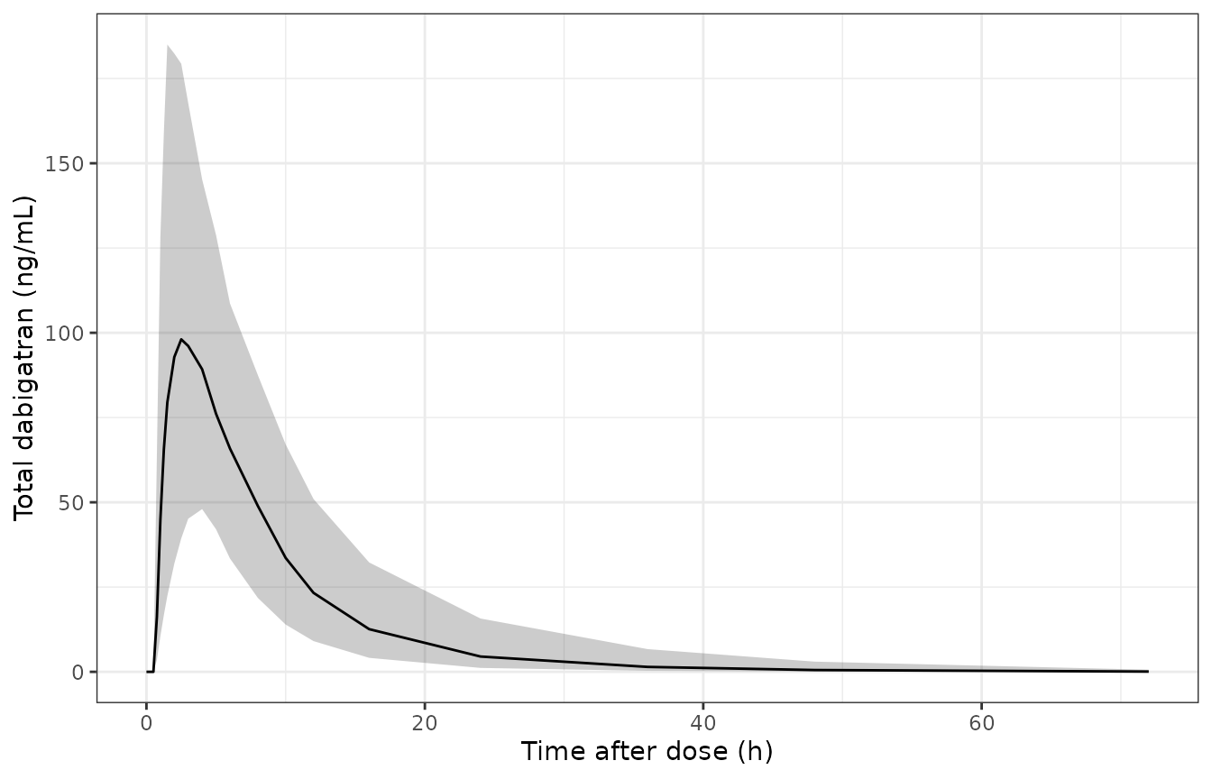
Simulated total dabigatran after a single 150 mg dose in healthy volunteers (median and 90% prediction interval of the individual predictions); cf. Liu 2022 Supplementary Figure 3A.
NCA of the simulated healthy volunteers
conc_hv <- sim_hv |>
  filter(!is.na(Cc)) |>
  select(id, time, Cc, treatment)
dose_hv <- ev_hv |>
  filter(evid == 1) |>
  select(id, time, amt, treatment)
o_conc <- PKNCA::PKNCAconc(conc_hv, Cc ~ time | treatment + id)
o_dose <- PKNCA::PKNCAdose(dose_hv, amt ~ time | treatment + id)
o_data <- PKNCA::PKNCAdata(
  o_conc, o_dose,
  intervals = data.frame(start = 0, end = Inf, cmax = TRUE, tmax = TRUE,
                         aucinf.obs = TRUE, half.life = TRUE)
)
nca_hv <- PKNCA::pk.nca(o_data)
summary(nca_hv)
#>  start end          treatment   N       cmax              tmax   half.life
#>      0 Inf 150 mg single dose 118 105 [41.3] 2.75 [1.25, 8.00] 8.66 [1.08]
#>  aucinf.obs
#>  886 [40.9]
#>
#> Caption: cmax, aucinf.obs: geometric mean and geometric coefficient of variation; tmax: median and range; half.life: arithmetic mean and standard deviation; N: number of subjects
The paper reports no NCA for this cohort, so there is no reference table. As an internal check, the median AUC0-inf should be close to dose / (CL/F) at the median covariates: 150 mg / 166 L/h = 904 ng*h/mL.
Steady-state check against the Discussion simulation
The paper’s Discussion reports median simulated concentrations of
48.68 ng/mL at 12 h and 168.22 ng/mL at 14 h for 75-year-old patients on
150 mg twice daily. A cohort of 200 such patients is simulated with the
integrated model, with HDL at its reference value, since the paper does
not state it. The concentrations at 12 h and 14 h are taken as
clast.obs over the intervals 0-12 h and 12-14 h.
n_pt <- 200
t_pt <- sort(unique(c(seq(0, 24, by = 0.5), 14)))
ev_pt <- bind_rows(
  tidyr::expand_grid(id = seq_len(n_pt), time = c(0, 12)) |>
    mutate(evid = 1L, amt = 150, cmt = "depot", dvid = NA_integer_),
  tidyr::expand_grid(id = seq_len(n_pt), time = t_pt) |>
    mutate(evid = 0L, amt = 0, cmt = NA_character_, dvid = 1L)
) |>
  mutate(AGE = 75, HDLC = 1.42, CRCL = 30, treatment = "150 mg BID, age 75") |>
  arrange(id, time, desc(evid))
sim_pt <- rxode2::rxSolve(mod, ev_pt, keep = "treatment", useLinCmt = FALSE) |>
  as.data.frame()

conc_pt <- sim_pt |> filter(!is.na(Cc)) |> select(id, time, Cc, treatment)
dose_pt <- ev_pt |> filter(evid == 1) |> select(id, time, amt, treatment)
nca_pt <- PKNCA::pk.nca(PKNCA::PKNCAdata(
  PKNCA::PKNCAconc(conc_pt, Cc ~ time | treatment + id),
  PKNCA::PKNCAdose(dose_pt, amt ~ time | treatment + id),
  intervals = data.frame(start = c(0, 12), end = c(12, 14), clast.obs = TRUE)
))
ref_pt <- data.frame(treatment = "150 mg BID, age 75", end = c(12, 14),
                     clast.obs = c(48.68, 168.22))
tbl_pt <- nlmixr2lib::ncaComparisonTable(
  nca_pt, ref_pt, by = c("treatment", "end"),
  units = c(clast.obs = "ng/mL")
)
tbl_pt |>
  rename(`Sampling time (h)` = end) |>
knitr::kable()| NCA parameter | treatment | Sampling time (h) | Reference | Simulated | % diff |
|---|---|---|---|---|---|
| Clast (ng/mL) | 150 mg BID, age 75 | 12 | 48.7 | 48.6 | -0.3% |
| Clast (ng/mL) | 150 mg BID, age 75 | 14 | 168 | 174 | +3.6% |
Biomarker peaks and troughs (Results, “Exposure simulation”)
Each scenario below has the same 200 virtual patients (identical random effects, so the scenarios differ only in CrCL and dose). The paper reports means and 95% confidence intervals from 1,000 replicates, at 2 h (peak) and 0.05 h (trough) after the first dose. Age and HDL are held at the reference values, which the reproduced typical-patient trough of aPTT indicates.
scen <- tribble(
  ~scenario,          ~CRCL,  ~amt,
  "typical, 150 mg",  120.18, 150,
  "CrCL 50, 150 mg",  50,     150,
  "CrCL 30, 110 mg",  30,     110
)
sim_pd <- lapply(seq_len(nrow(scen)), function(i) {
  ev_i <- bind_rows(
    data.frame(id = seq_len(n_pt), time = 0, evid = 1L, amt = scen$amt[i],
               cmt = "depot", dvid = NA_integer_),
    tidyr::expand_grid(id = seq_len(n_pt), time = c(0.05, seq(0.5, 12, by = 0.5))) |>
      mutate(evid = 0L, amt = 0, cmt = NA_character_, dvid = 1L)
  ) |>
    mutate(CRCL = scen$CRCL[i], AGE = 22, HDLC = 1.42) |>
    arrange(id, time, desc(evid))
  # Same seed and event layout in every scenario -> identical eta draws.
  rxode2::rxSetSeed(20221028)
  rxode2::rxSolve(mod, ev_i, useLinCmt = FALSE) |>
    as.data.frame() |>
    mutate(scenario = scen$scenario[i])
}) |>
  bind_rows()

pd_sum <- sim_pd |>
  filter(time %in% c(0.05, 2)) |>
  select(scenario, time, aPTT, PT, antiFIIa) |>
  pivot_longer(c(aPTT, PT, antiFIIa), names_to = "marker") |>
  group_by(scenario, marker, time) |>
  summarise(sim_mean = mean(value), .groups = "drop") |>
  mutate(what = ifelse(time == 2, "peak", "trough")) |>
  select(-time) |>
  left_join(
    paper_pd |>
      pivot_longer(c(peak, trough), names_to = "what", values_to = "paper"),
    by = c("scenario", "marker", "what")
  ) |>
  mutate(`% diff` = round(100 * (sim_mean / paper - 1), 1),
         sim_mean = signif(sim_mean, 4))
pd_sum |>
  arrange(match(scenario, scen$scenario), marker, what) |>
  select(scenario, marker, what, paper, sim_mean, `% diff`) |>
  rename(Scenario = scenario, Marker = marker, Statistic = what,
         `Liu 2022 (mean)` = paper, `Simulated (mean)` = sim_mean) |>
knitr::kable()| Scenario | Marker | Statistic | Liu 2022 (mean) | Simulated (mean) | % diff |
|---|---|---|---|---|---|
| typical, 150 mg | PT | peak | 13.01 | 12.78 | -1.8 |
| typical, 150 mg | PT | trough | 11.79 | 11.80 | 0.1 |
| typical, 150 mg | aPTT | peak | 40.20 | 38.84 | -3.4 |
| typical, 150 mg | aPTT | trough | 32.49 | 32.22 | -0.8 |
| typical, 150 mg | antiFIIa | peak | 130.58 | 118.40 | -9.3 |
| typical, 150 mg | antiFIIa | trough | 20.13 | 20.50 | 1.8 |
| CrCL 50, 150 mg | PT | peak | 18.97 | 17.56 | -7.4 |
| CrCL 50, 150 mg | PT | trough | 11.79 | 11.80 | 0.1 |
| CrCL 50, 150 mg | aPTT | peak | 48.13 | 46.81 | -2.7 |
| CrCL 50, 150 mg | aPTT | trough | 40.42 | 40.18 | -0.6 |
| CrCL 50, 150 mg | antiFIIa | peak | 377.68 | 340.40 | -9.9 |
| CrCL 50, 150 mg | antiFIIa | trough | 20.13 | 20.50 | 1.8 |
| CrCL 30, 110 mg | PT | peak | 26.59 | 23.65 | -11.0 |
| CrCL 30, 110 mg | PT | trough | 11.79 | 11.80 | 0.1 |
| CrCL 30, 110 mg | aPTT | peak | 51.58 | 50.56 | -2.0 |
| CrCL 30, 110 mg | aPTT | trough | 45.98 | 45.71 | -0.6 |
| CrCL 30, 110 mg | antiFIIa | peak | 543.18 | 488.00 | -10.2 |
| CrCL 30, 110 mg | antiFIIa | trough | 20.13 | 20.50 | 1.8 |
The troughs reproduce the baselines, and the peaks are within about 10% of the paper’s means. For the typical patient, the paper’s reported 95% CI for the anti-FIIa peak is 120.40-140.77 ng/mL. The slope IIV of PT (omega^2 1.25) and anti-FIIa (omega^2 1.1) is heavy-tailed, so the mean of 200 subjects moves by roughly 10% between random draws. That level is set by the typical-patient row, and the CrCL scenarios then follow from the deterministic ratios checked above. The aPTT peak is the least well reproduced, at about 4% low. The paper notes that its aPTT simulation was the least accurate of the three biomarkers (“poorer simulation accuracy than for PT and anti-FIIa activity”, Discussion).
# Baselines carry no drug and no CrCL-dependent IIV for PT / anti-FIIa:
# the trough means equal the Table 2 baselines.
tr <- pd_sum |> filter(what == "trough")
stopifnot(abs(median(tr$`% diff`)) < 5)
# Peaks: centre of the nine peak comparisons. The slope IIV is heavy-tailed,
# so individual stochastic means are not asserted.
pk <- pd_sum |> filter(what == "peak")
stopifnot(abs(median(pk$`% diff`)) < 15)
sim_pd |>
  select(scenario, time, aPTT, PT, antiFIIa) |>
  pivot_longer(c(aPTT, PT, antiFIIa), names_to = "marker") |>
  group_by(scenario, marker, time) |>
  summarise(med = median(value), .groups = "drop") |>
  ggplot(aes(time, med, colour = scenario)) +
  geom_line() +
  facet_wrap(~marker, scales = "free_y") +
  labs(x = "Time after first dose (h)", y = "Median prediction", colour = NULL) +
  theme_bw() +
  theme(legend.position = "bottom")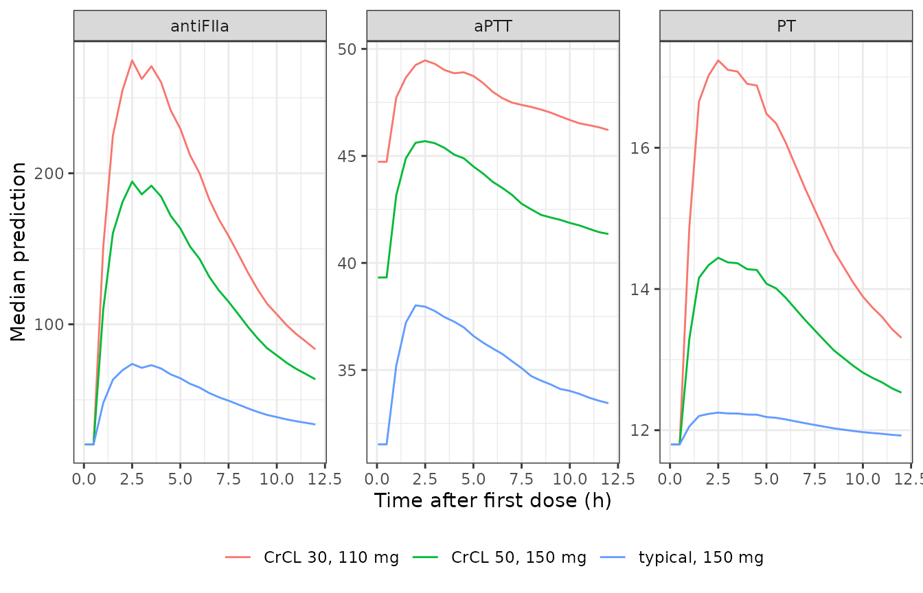
Simulated biomarker time courses after the first dose for the three scenarios (median of the individual predictions); cf. Liu 2022 Figure 5.
Healthy-volunteer versus integrated PD
The healthy-volunteer PD model (no covariates) and the integrated model at the healthy-volunteer reference covariates differ only through their re-estimated baselines and slopes. The typical-value comparison after a single 150 mg dose is below.
ev_one <- bind_rows(
  data.frame(id = 1L, time = 0, evid = 1L, amt = 150, cmt = "depot",
             dvid = NA_integer_),
  data.frame(id = 1L, time = c(0, 2, 8, 12), evid = 0L, amt = 0,
             cmt = NA_character_, dvid = 1L)
) |>
  mutate(AGE = 22, HDLC = 1.42, CRCL = 120.18) |>
  arrange(time, desc(evid))
tv <- function(m, lab) {
  as.data.frame(rxode2::rxSolve(m, ev_one, omega = NA, sigma = NA,
                                useLinCmt = FALSE)) |>
    select(time, Cc, aPTT, PT, antiFIIa) |>
    mutate(model = lab)
}
bind_rows(tv(mod_hv, "healthy volunteers"), tv(mod, "integrated")) |>
  mutate(across(c(Cc, aPTT, PT, antiFIIa), \(x) signif(x, 4))) |>
  rename(`Time (h)` = time, `Cc (ng/mL)` = Cc, `aPTT (s)` = aPTT,
         `PT (s)` = PT, `anti-FIIa (ng/mL)` = antiFIIa, Model = model) |>
knitr::kable()| Time (h) | Cc (ng/mL) | aPTT (s) | PT (s) | anti-FIIa (ng/mL) | Model |
|---|---|---|---|---|---|
| 0 | 0.00 | 30.40 | 11.70 | 14.90 | healthy volunteers |
| 2 | 109.50 | 40.38 | 12.62 | 83.68 | healthy volunteers |
| 8 | 47.48 | 34.73 | 12.10 | 44.72 | healthy volunteers |
| 12 | 21.54 | 32.36 | 11.88 | 28.43 | healthy volunteers |
| 0 | 0.00 | 32.00 | 11.80 | 20.50 | integrated |
| 2 | 109.50 | 39.04 | 12.46 | 82.05 | integrated |
| 8 | 47.48 | 35.05 | 12.08 | 47.19 | integrated |
| 12 | 21.54 | 33.39 | 11.93 | 32.61 | integrated |