Multi-objective Pareto-front popPK models for 17-DMAG / alvespimycin (Li 2026)
Source:vignettes/articles/Li_2026_alvespimycin.Rmd
Li_2026_alvespimycin.RmdModel and source
Li et al. (2026) do not develop a single drug model. They apply multi-objective optimization – the non-dominated sorting genetic algorithm II (NSGA-II), as implemented in pyDarwin – to population PK model selection, minimising the objective function value (OFV) and the number of estimated parameters (NEP) simultaneously. The output of such a search is not one model but a Pareto front: a set of non-dominated structures, each of which is the best available fit at its own level of parsimony.
Four data sets are searched (17-DMAG, ziprasidone, clozapine,
quetiapine), but full parameter estimates with uncertainty are reported
for exactly four models: the 17-DMAG (alvespimycin) non-dominated
solutions selected for the prediction-corrected VPC comparison, at NEP =
5, 9, 11 and 16 (Supplementary Table S2, models a-d). Those four models
are the four .R files packaged here. Supplementary Tables
S3-S6 tabulate the remaining non-dominated structures for all four
compounds, but report only OFV, structure and diagnostics – no parameter
values – so they are not extractable.
liModels <- c(
  "Li_2026_alvespimycin_nep5",
  "Li_2026_alvespimycin_nep9",
  "Li_2026_alvespimycin_nep11",
  "Li_2026_alvespimycin_nep16"
)- Article: https://doi.org/10.1007/s10928-026-10036-9
- Supplementary information (Tables S1-S7, including the parameter table S2): https://doi.org/10.1007/s10928-026-10036-9
- Predecessor study that deposits the pyDarwin template, token and final control files for this same 17-DMAG search space: https://doi.org/10.1007/s10928-024-09932-9
These are machine-search structures from a model-selection
methods study, not expert-developed final models. The same
17-DMAG data set was analysed by a conventional stepwise search in
Aregbe et al. (2012), which is packaged separately here as
Aregbe_2012_alvespimycin. A reader who wants “the”
published population PK model for 17-DMAG should go to that file; what
these four files reproduce is Li 2026’s own reported result – a family
of models that trades fit against complexity.
for (nm in liModels) {
  m <- rxode2::rxode(readModelDb(nm))
  cat("\n## ", nm, "\n\n", sep = "")
  cat("* Description: ", m$description, "\n", sep = "")
}
#> ℹ parameter labels from comments will be replaced by 'label()'
Li_2026_alvespimycin_nep5
- Description: One-compartment population PK model for the heat shock protein 90 inhibitor 17-DMAG (alvespimycin) given as an IV infusion to adult patients with advanced solid tumors, recovered as the most parsimonious non-dominated solution (5 estimated parameters, OFV 9813.4) on the NSGA-II multi-objective Pareto front of Li 2026, with first-order elimination, log-normal IIV on CL and Vc, and an exponential residual error model. This is a machine-search model structure from a multi-objective model-selection study, not an expert-developed final model.
#> ℹ parameter labels from comments will be replaced by 'label()'
#> Warning: some etas defaulted to non-mu referenced, possible parsing error: etaiov_q_1, etaiov_q_2, etaiov_q_3
#> as a work-around try putting the mu-referenced expression on a simple line
Li_2026_alvespimycin_nep9
- Description: Two-compartment population PK model for the heat shock protein 90 inhibitor 17-DMAG (alvespimycin) given as an IV infusion to adult patients with advanced solid tumors, recovered as the 9-estimated-parameter non-dominated solution (OFV 8335.4) on the NSGA-II multi-objective Pareto front of Li 2026, with first-order elimination, log-normal IIV on CL, Vc and Vp, between-occasion variability on inter-compartmental clearance, and an exponential residual error model. This is a machine-search model structure from a multi-objective model-selection study, not an expert-developed final model.
#> ℹ parameter labels from comments will be replaced by 'label()'
#> Warning: some etas defaulted to non-mu referenced, possible parsing error: etaiov_cl_1, etaiov_cl_2, etaiov_cl_3
#> as a work-around try putting the mu-referenced expression on a simple line
Li_2026_alvespimycin_nep11
- Description: Three-compartment population PK model for the heat shock protein 90 inhibitor 17-DMAG (alvespimycin) given as an IV infusion to adult patients with advanced solid tumors, recovered as the 11-estimated-parameter non-dominated solution (OFV 8166.5) on the NSGA-II multi-objective Pareto front of Li 2026, with first-order elimination, log-normal IIV on CL, Vc and Vp, between-occasion variability on clearance, and an exponential residual error model. This is a machine-search model structure from a multi-objective model-selection study, not an expert-developed final model.
#> ℹ parameter labels from comments will be replaced by 'label()'
#> Warning: some etas defaulted to non-mu referenced, possible parsing error: etaiov_cl_1, etaiov_cl_2, etaiov_cl_3, etaiov_vc_1, etaiov_vc_2, etaiov_vc_3, etaiov_q_1, etaiov_q_2, etaiov_q_3
#> as a work-around try putting the mu-referenced expression on a simple line
Li_2026_alvespimycin_nep16
- Description: Three-compartment population PK model for the heat shock protein 90 inhibitor 17-DMAG (alvespimycin) given as an IV infusion to adult patients with advanced solid tumors, recovered as the 16-estimated-parameter non-dominated solution (OFV 8041.3) on the NSGA-II multi-objective Pareto front of Li 2026 and identical to the optimum found by the single-objective hybrid genetic algorithm, with first-order elimination, a power effect of body weight on central volume, log-normal IIV on CL, Vc, Vp and Q3, between-occasion variability on CL, Vc and Q2, and a combined residual error model. This is a machine-search model structure from a multi-objective model-selection study, not an expert-developed final model.
Population
All four models are fit to the same 17-DMAG data set: 66 adult patients with advanced solid tumours contributing 951 plasma concentrations, sampled relatively richly (more than 15 samples per participant on average) over up to 102 h. Demographics are from Li 2026 Supplementary Table S1, DMAG panel.
pop <- readModelDb("Li_2026_alvespimycin_nep16")()$population
#> Warning: some etas defaulted to non-mu referenced, possible parsing error: etaiov_cl_1, etaiov_cl_2, etaiov_cl_3, etaiov_vc_1, etaiov_vc_2, etaiov_vc_3, etaiov_q_1, etaiov_q_2, etaiov_q_3
#> as a work-around try putting the mu-referenced expression on a simple line
data.frame(
  Field = c("Species", "Subjects", "Observations", "Age", "Weight",
            "Female", "Disease", "Dose"),
  Value = c(
    pop$species,
    format(pop$n_subjects), format(pop$n_observations),
    pop$age_range, pop$weight_range,
    paste0(pop$sex_female_pct, "%"),
    pop$disease_state, pop$dose_range
  )
) |>
knitr::kable()| Field | Value |
|---|---|
| Species | human |
| Subjects | 66 |
| Observations | 951 |
| Age | 28-82 years (median 63) |
| Weight | 48.2-136.5 kg (median 80.3) |
| Female | 38% |
| Disease | Adult patients with advanced solid tumors. |
| Dose | IV infusion of 17-DMAG; median 33, range 2.2-413 per the dose column of Li 2026 Table 1 (see notes on the unit of that column). |
Source trace
Every ini() value in the four model files, and every
non-obvious structural choice in model(), with the source
location it was taken from.
sourceTrace <- tibble::tribble(
  ~Model,  ~Item, ~Source,
  "all",   "Structural compartment count (1 / 2 / 3 / 3)", "Li 2026 Table S3, DMAG NSGA-II rows, `COM` column at NEP = 5 / 9 / 11 / 16",
  "all",   "BSV and BOV placement", "Li 2026 Table S3, DMAG NSGA-II rows, `BSV` and `BOV` columns",
  "all",   "Residual error family (prop / prop / prop / comb)", "Li 2026 Table S3, DMAG NSGA-II rows, `RUV` column",
  "all",   "`prop` token is `F*EXP(EPS)`; `comb` token is `F*EXP(EPS(1)) + EPS(2)`", "Li 2024 Supplementary Material 2 (pyDarwin token file), `RESERR` entry",
  "all",   "Three occasions for BOV multiplexing", "Li 2024 Supplementary Material 4 (final control stream), `$PK`: `IF(OCC.EQ.1) ... IF(OCC.EQ.3)`",
  "all",   "Concentration on the ng/mL scale (`Cc = 1000 * central / vc`)", "Li 2024 Supplementary Material 4, `S1 = V1` with no scaling factor; Li 2026 Figure 2 pcVPC concentration axis runs to about 2500",
  "all",   "Population demographics", "Li 2026 Table S1, DMAG panel; Li 2026 Table 1 (66 subjects, 951 observations)",
  "nep5",  "CL = 8.41 L/hr, V = 98.4 L", "Li 2026 Table S2, Model a (NEP = 5, OFV = 9813.4)",
  "nep5",  "BSV CL 35.8%, BSV V 31.3%", "Li 2026 Table S2, Model a",
  "nep5",  "Residual 0.214 (variance) -> expSd 0.4626", "Li 2026 Table S2, Model a",
  "nep9",  "CL = 9.65, Q = 61.8, V = 37.8, V2 = 127", "Li 2026 Table S2, Model b (NEP = 9, OFV = 8335.4)",
  "nep9",  "BSV CL 43.4%, V 51.9%, V2 48.4%; BOV Q 45.9%", "Li 2026 Table S2, Model b",
  "nep9",  "Residual 0.034 (variance) -> expSd 0.1844", "Li 2026 Table S2, Model b",
  "nep11", "CL = 9.26, Q2 = 81.8, Q3 = 9.47, V = 28.1, V2 = 75.6, V3 = 85.3", "Li 2026 Table S2, Model c (NEP = 11, OFV = 8166.5)",
  "nep11", "BSV CL 43.5%, V 70.2%, V2 63.3%; BOV CL 27.7%", "Li 2026 Table S2, Model c",
  "nep11", "Residual 0.029 (variance) -> expSd 0.1703", "Li 2026 Table S2, Model c",
  "nep16", "CL = 8.64, Q2 = 79.3, Q3 = 9.74, V = 29.1, V2 = 71.9, V3 = 136", "Li 2026 Table S2, Model d (NEP = 16, OFV = 8041.3)",
  "nep16", "Weight-on-volume power exponent 1.31", "Li 2026 Table S2, Model d",
  "nep16", "Weight centred on 81 kg", "Li 2024 Supplementary Material 1 and 4: `CWTKGONE = WT/81`, `TVV = THETA(1)*CWTKGONE**THETA(7)`",
  "nep16", "BSV CL 50.3%, V 42.9%, V2 58.7%, Q3 75.8%", "Li 2026 Table S2, Model d",
  "nep16", "BOV CL 30.3%, V 31.1%, Q2 28.6%", "Li 2026 Table S3 (`BOV` = `V, CL, Q2`) and Li 2024 parameter table; see Errata",
  "nep16", "Residual 0.017 and 14.7 (variances) -> propSd 0.1304, addSd 3.834 ng/mL", "Li 2026 Table S2, Model d"
)
knitr::kable(sourceTrace)| Model | Item | Source |
|---|---|---|
| all | Structural compartment count (1 / 2 / 3 / 3) | Li 2026 Table S3, DMAG NSGA-II rows, COM
column at NEP = 5 / 9 / 11 / 16 |
| all | BSV and BOV placement | Li 2026 Table S3, DMAG NSGA-II rows, BSV
and BOV columns |
| all | Residual error family (prop / prop / prop / comb) | Li 2026 Table S3, DMAG NSGA-II rows, RUV
column |
| all |
prop token is F*EXP(EPS);
comb token is F*EXP(EPS(1)) + EPS(2)
|
Li 2024 Supplementary Material 2 (pyDarwin token file),
RESERR entry |
| all | Three occasions for BOV multiplexing | Li 2024 Supplementary Material 4 (final control
stream), $PK:
IF(OCC.EQ.1) ... IF(OCC.EQ.3)
|
| all | Concentration on the ng/mL scale
(Cc = 1000 * central / vc) |
Li 2024 Supplementary Material 4, S1 = V1
with no scaling factor; Li 2026 Figure 2 pcVPC concentration axis runs
to about 2500 |
| all | Population demographics | Li 2026 Table S1, DMAG panel; Li 2026 Table 1 (66 subjects, 951 observations) |
| nep5 | CL = 8.41 L/hr, V = 98.4 L | Li 2026 Table S2, Model a (NEP = 5, OFV = 9813.4) |
| nep5 | BSV CL 35.8%, BSV V 31.3% | Li 2026 Table S2, Model a |
| nep5 | Residual 0.214 (variance) -> expSd 0.4626 | Li 2026 Table S2, Model a |
| nep9 | CL = 9.65, Q = 61.8, V = 37.8, V2 = 127 | Li 2026 Table S2, Model b (NEP = 9, OFV = 8335.4) |
| nep9 | BSV CL 43.4%, V 51.9%, V2 48.4%; BOV Q 45.9% | Li 2026 Table S2, Model b |
| nep9 | Residual 0.034 (variance) -> expSd 0.1844 | Li 2026 Table S2, Model b |
| nep11 | CL = 9.26, Q2 = 81.8, Q3 = 9.47, V = 28.1, V2 = 75.6, V3 = 85.3 | Li 2026 Table S2, Model c (NEP = 11, OFV = 8166.5) |
| nep11 | BSV CL 43.5%, V 70.2%, V2 63.3%; BOV CL 27.7% | Li 2026 Table S2, Model c |
| nep11 | Residual 0.029 (variance) -> expSd 0.1703 | Li 2026 Table S2, Model c |
| nep16 | CL = 8.64, Q2 = 79.3, Q3 = 9.74, V = 29.1, V2 = 71.9, V3 = 136 | Li 2026 Table S2, Model d (NEP = 16, OFV = 8041.3) |
| nep16 | Weight-on-volume power exponent 1.31 | Li 2026 Table S2, Model d |
| nep16 | Weight centred on 81 kg | Li 2024 Supplementary Material 1 and 4:
CWTKGONE = WT/81,
TVV = THETA(1)*CWTKGONE**THETA(7)
|
| nep16 | BSV CL 50.3%, V 42.9%, V2 58.7%, Q3 75.8% | Li 2026 Table S2, Model d |
| nep16 | BOV CL 30.3%, V 31.1%, Q2 28.6% | Li 2026 Table S3 (BOV =
V, CL, Q2) and Li 2024 parameter table; see Errata |
| nep16 | Residual 0.017 and 14.7 (variances) -> propSd 0.1304, addSd 3.834 ng/mL | Li 2026 Table S2, Model d |
Replicating the Pareto front (Figure 1a)
Figure 1a of Li 2026 plots the DMAG Pareto front: OFV against NEP, for the NSGA-II search with and without a local downhill step. Those coordinates are transcribed directly from Supplementary Table S3 – no simulation is involved, so the reproduction is exact and the four models packaged here can be located on the front.
paretoNoDownhill <- tibble::tribble(
  ~nep, ~ofv,
  5, 9813.4,  6, 9769.9,  7, 8799.4,  8, 8452.4,  9, 8335.4, 10, 8238.3,
  11, 8166.5, 12, 8134.1, 13, 8101.6, 14, 8065.6, 15, 8056.9, 16, 8041.3,
  17, 8041.2, 18, 8040.8, 19, 8035.1, 21, 8034.6, 22, 8034.5
)
paretoDownhill <- tibble::tribble(
  ~nep, ~ofv,
  5, 9813.4,  6, 9769.9,  7, 8799.4,  8, 8452.4,  9, 8335.4, 10, 8238.3,
  11, 8166.5, 12, 8134.1, 13, 8094.8, 14, 8065.6, 15, 8050.9, 16, 8041.3,
  17, 8032.7, 18, 8029.9, 19, 8027.4, 20, 8025.0, 21, 8024.8, 22, 8024.7,
  23, 8024.6
)
pareto <- dplyr::bind_rows(
  dplyr::mutate(paretoNoDownhill, search = "NSGA-II, no downhill"),
  dplyr::mutate(paretoDownhill,   search = "NSGA-II, with downhill")
)
packaged <- dplyr::filter(paretoDownhill, nep %in% c(5, 9, 11, 16))

ggplot2::ggplot(pareto, ggplot2::aes(nep, ofv, colour = search)) +
  ggplot2::geom_point(size = 2) +
  ggplot2::geom_point(
    data = packaged, ggplot2::aes(nep, ofv),
    inherit.aes = FALSE, shape = 21, size = 5, stroke = 1.1
  ) +
  ggplot2::labs(
    x = "Number of estimated parameters (NEP)",
    y = "OFV (-2LL)", colour = NULL,
    caption = "Replicates Figure 1a of Li 2026 (values from Table S3). Circled points are the four models packaged here."
  ) +
  ggplot2::theme_bw() +
  ggplot2::theme(legend.position = "bottom")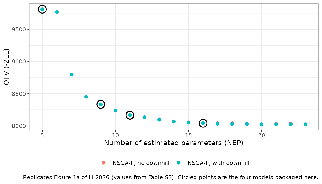
stopifnot(
  # The abstract states 17 non-dominated DMAG solutions without downhill search.
  nrow(paretoNoDownhill) == 17L,
  # The Results text gives the OFV and NEP ranges for both searches.
  min(paretoNoDownhill$nep) == 5L, max(paretoNoDownhill$nep) == 22L,
  abs(max(paretoNoDownhill$ofv) - 9813.4) < 1e-6,
  abs(min(paretoNoDownhill$ofv) - 8034.5) < 1e-6,
  min(paretoDownhill$nep) == 5L, max(paretoDownhill$nep) == 23L,
  abs(min(paretoDownhill$ofv) - 8024.6) < 1e-6,
  # A Pareto front must be monotone: OFV never increases as NEP grows.
  all(diff(paretoNoDownhill$ofv) <= 0),
  all(diff(paretoDownhill$ofv) <= 0)
)
Typical-value profiles
The paper’s own subjective comparison (Figure 2a-d) is a pcVPC of the four models against the observed data, which is not redistributed with this package. What can be reproduced without the data is the structural claim the figure is used to make: that adding compartments progressively changes the shape of the predicted profile, most obviously in the distribution and terminal phases.
A single 1 h IV infusion of 63 mg (the Li 2026 Table 1 median of 33 scaled by a 1.9 m^2 body surface area, since Aregbe 2012 reports that dose column in mg/m^2) is simulated at the typical value of every parameter, with all random effects zeroed.
rxode2::rxSetSeed(1042)

typicalEvents <- rxode2::et(amt = 63, dur = 1, cmt = "central") |>
  rxode2::et(seq(0, 120, by = 0.25), cmt = "central") |>
  as.data.frame()
typicalEvents$WT  <- 81
typicalEvents$OCC <- 1

typicalProfiles <-
  lapply(liModels, function(nm) {
    ui <- rxode2::rxode(readModelDb(nm))
    out <- rxode2::rxSolve(
      rxode2::zeroRe(ui), typicalEvents, returnType = "data.frame"
    )
    out$model <- nm
    out[, c("model", "time", "Cc")]
  }) |>
  dplyr::bind_rows() |>
  dplyr::mutate(model = factor(model, levels = liModels))
#> ℹ parameter labels from comments will be replaced by 'label()'
#> ℹ omega/sigma items treated as zero: 'etalcl', 'etalvc'
#> ℹ parameter labels from comments will be replaced by 'label()'
#> Warning: some etas defaulted to non-mu referenced, possible parsing error: etaiov_q_1, etaiov_q_2, etaiov_q_3
#> as a work-around try putting the mu-referenced expression on a simple line
#> Warning: some etas defaulted to non-mu referenced, possible parsing error: etaiov_q_1, etaiov_q_2, etaiov_q_3
#> as a work-around try putting the mu-referenced expression on a simple line
#> ℹ omega/sigma items treated as zero: 'etalcl', 'etalvc', 'etalvp', 'etaiov_q_1', 'etaiov_q_2', 'etaiov_q_3'
#> ℹ parameter labels from comments will be replaced by 'label()'
#> Warning: some etas defaulted to non-mu referenced, possible parsing error: etaiov_cl_1, etaiov_cl_2, etaiov_cl_3
#> as a work-around try putting the mu-referenced expression on a simple line
#> Warning: some etas defaulted to non-mu referenced, possible parsing error: etaiov_cl_1, etaiov_cl_2, etaiov_cl_3
#> as a work-around try putting the mu-referenced expression on a simple line
#> ℹ omega/sigma items treated as zero: 'etalcl', 'etalvc', 'etalvp', 'etaiov_cl_1', 'etaiov_cl_2', 'etaiov_cl_3'
#> ℹ parameter labels from comments will be replaced by 'label()'
#> Warning: some etas defaulted to non-mu referenced, possible parsing error: etaiov_cl_1, etaiov_cl_2, etaiov_cl_3, etaiov_vc_1, etaiov_vc_2, etaiov_vc_3, etaiov_q_1, etaiov_q_2, etaiov_q_3
#> as a work-around try putting the mu-referenced expression on a simple line
#> Warning: some etas defaulted to non-mu referenced, possible parsing error: etaiov_cl_1, etaiov_cl_2, etaiov_cl_3, etaiov_vc_1, etaiov_vc_2, etaiov_vc_3, etaiov_q_1, etaiov_q_2, etaiov_q_3
#> as a work-around try putting the mu-referenced expression on a simple line
#> ℹ omega/sigma items treated as zero: 'etalcl', 'etalvc', 'etalvp', 'etalq2', 'etaiov_cl_1', 'etaiov_cl_2', 'etaiov_cl_3', 'etaiov_vc_1', 'etaiov_vc_2', 'etaiov_vc_3', 'etaiov_q_1', 'etaiov_q_2', 'etaiov_q_3'

ggplot2::ggplot(typicalProfiles, ggplot2::aes(time, Cc, colour = model)) +
  ggplot2::geom_line(linewidth = 0.8) +
  ggplot2::scale_y_log10() +
  ggplot2::labs(
    x = "Time (h)", y = "Plasma 17-DMAG (ng/mL)", colour = NULL,
    caption = "Typical-value profiles after a 1 h, 63 mg IV infusion. Compare the shape progression in Figure 2a-d of Li 2026."
  ) +
  ggplot2::theme_bw() +
  ggplot2::theme(legend.position = "bottom")
#> Warning in ggplot2::scale_y_log10(): log-10 transformation introduced infinite
#> values.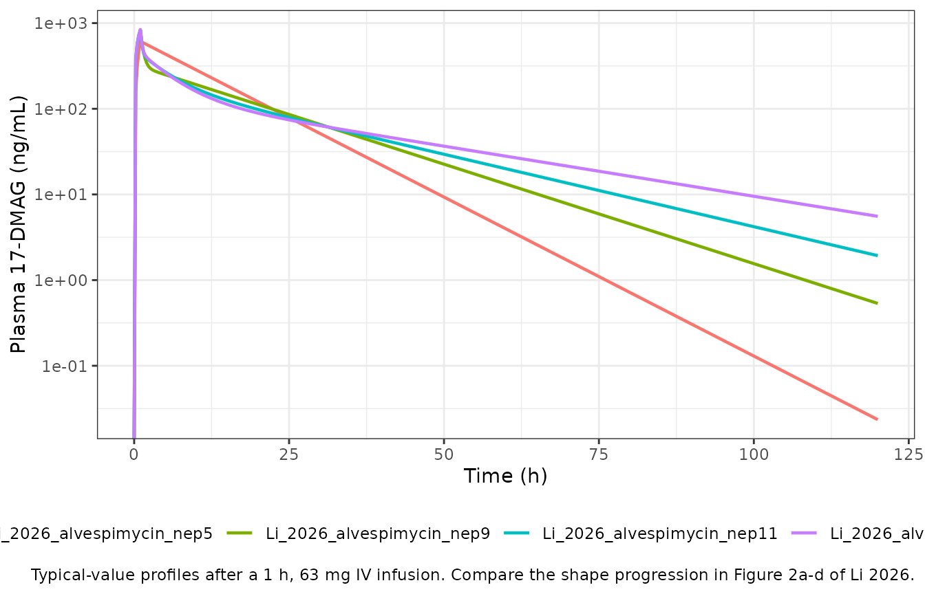
terminal <-
  typicalProfiles |>
  dplyr::filter(time == 120) |>
  dplyr::arrange(model)

# Structural claim of Figure 2: more compartments means more drug still
# circulating at the end of the observation window, because the deep
# peripheral compartments release drug back slowly. Deterministic (zeroRe),
# so an exact ordering is the right assertion.
stopifnot(
  nrow(terminal) == 4L,
  all(diff(terminal$Cc) > 0),
  # The one-compartment model has by far the largest central volume, so its
  # early concentrations are the lowest of the four.
  which.min(
    typicalProfiles$Cc[typicalProfiles$time == 1]
  ) == 1L
)
Structural identity checks
For an IV bolus at the typical value of every parameter, non-compartmental analysis must recover the model’s own clearance and steady-state volume exactly, up to numerical integration error. Both sides of this comparison use the same parameters, so the difference is pure numerical error and a tight bound is the correct assertion.
bolusEvents <- rxode2::et(amt = 63, cmt = "central") |>
  rxode2::et(c(seq(0, 2, by = 0.02), seq(2.5, 24, by = 0.5),
               seq(25, 240, by = 2), seq(244, 720, by = 4)),
             cmt = "central") |>
  as.data.frame()
bolusEvents$WT  <- 81
bolusEvents$OCC <- 1

bolusConc <-
  lapply(liModels, function(nm) {
    ui <- rxode2::rxode(readModelDb(nm))
    out <- rxode2::rxSolve(
      rxode2::zeroRe(ui), bolusEvents, returnType = "data.frame"
    )
    data.frame(model = nm, id = 1L, time = out$time, Cc = out$Cc)
  }) |>
  dplyr::bind_rows() |>
  dplyr::filter(!is.na(Cc))
#> ℹ parameter labels from comments will be replaced by 'label()'
#> ℹ omega/sigma items treated as zero: 'etalcl', 'etalvc'
#> ℹ parameter labels from comments will be replaced by 'label()'
#> Warning: some etas defaulted to non-mu referenced, possible parsing error: etaiov_q_1, etaiov_q_2, etaiov_q_3
#> as a work-around try putting the mu-referenced expression on a simple line
#> Warning: some etas defaulted to non-mu referenced, possible parsing error: etaiov_q_1, etaiov_q_2, etaiov_q_3
#> as a work-around try putting the mu-referenced expression on a simple line
#> ℹ omega/sigma items treated as zero: 'etalcl', 'etalvc', 'etalvp', 'etaiov_q_1', 'etaiov_q_2', 'etaiov_q_3'
#> ℹ parameter labels from comments will be replaced by 'label()'
#> Warning: some etas defaulted to non-mu referenced, possible parsing error: etaiov_cl_1, etaiov_cl_2, etaiov_cl_3
#> as a work-around try putting the mu-referenced expression on a simple line
#> Warning: some etas defaulted to non-mu referenced, possible parsing error: etaiov_cl_1, etaiov_cl_2, etaiov_cl_3
#> as a work-around try putting the mu-referenced expression on a simple line
#> ℹ omega/sigma items treated as zero: 'etalcl', 'etalvc', 'etalvp', 'etaiov_cl_1', 'etaiov_cl_2', 'etaiov_cl_3'
#> ℹ parameter labels from comments will be replaced by 'label()'
#> Warning: some etas defaulted to non-mu referenced, possible parsing error: etaiov_cl_1, etaiov_cl_2, etaiov_cl_3, etaiov_vc_1, etaiov_vc_2, etaiov_vc_3, etaiov_q_1, etaiov_q_2, etaiov_q_3
#> as a work-around try putting the mu-referenced expression on a simple line
#> Warning: some etas defaulted to non-mu referenced, possible parsing error: etaiov_cl_1, etaiov_cl_2, etaiov_cl_3, etaiov_vc_1, etaiov_vc_2, etaiov_vc_3, etaiov_q_1, etaiov_q_2, etaiov_q_3
#> as a work-around try putting the mu-referenced expression on a simple line
#> ℹ omega/sigma items treated as zero: 'etalcl', 'etalvc', 'etalvp', 'etalq2', 'etaiov_cl_1', 'etaiov_cl_2', 'etaiov_cl_3', 'etaiov_vc_1', 'etaiov_vc_2', 'etaiov_vc_3', 'etaiov_q_1', 'etaiov_q_2', 'etaiov_q_3'

bolusDose <- data.frame(
  model = liModels, id = 1L, time = 0, amt = 63
)

concObj <- PKNCA::PKNCAconc(bolusConc, Cc ~ time | model + id)
doseObj <- PKNCA::PKNCAdose(bolusDose, amt ~ time | model + id)
intervals <- data.frame(
  start = 0, end = Inf,
  cmax = TRUE, tmax = TRUE, auclast = TRUE, aucinf.obs = TRUE,
  aumcinf.obs = TRUE, half.life = TRUE
)
bolusNca <- PKNCA::pk.nca(PKNCA::PKNCAdata(concObj, doseObj, intervals = intervals))

bolusWide <-
  as.data.frame(bolusNca) |>
  dplyr::select(model, PPTESTCD, PPORRES) |>
  tidyr::pivot_wider(names_from = PPTESTCD, values_from = PPORRES)
PKNCA returns CL in dose units over
concentration units, i.e. mg / (ng/mL * h). One ng/mL is 1e-3 mg/L, so
multiplying by 1000 converts to L/h.
modelParams <-
  lapply(liModels, function(nm) {
    ini <- rxode2::rxode(readModelDb(nm))$iniDf
    tv  <- function(p) {
      v <- ini$est[ini$name == p]
      if (length(v) == 0) NA_real_ else exp(v)
    }
    data.frame(
      model  = nm,
      cl     = tv("lcl"),
      vss    = sum(c(tv("lvc"), tv("lvp"), tv("lvp2")), na.rm = TRUE),
      vc     = tv("lvc")
    )
  }) |>
  dplyr::bind_rows()
#> ℹ parameter labels from comments will be replaced by 'label()'
#> ℹ parameter labels from comments will be replaced by 'label()'
#> Warning: some etas defaulted to non-mu referenced, possible parsing error: etaiov_q_1, etaiov_q_2, etaiov_q_3
#> as a work-around try putting the mu-referenced expression on a simple line
#> ℹ parameter labels from comments will be replaced by 'label()'
#> Warning: some etas defaulted to non-mu referenced, possible parsing error: etaiov_cl_1, etaiov_cl_2, etaiov_cl_3
#> as a work-around try putting the mu-referenced expression on a simple line
#> ℹ parameter labels from comments will be replaced by 'label()'
#> Warning: some etas defaulted to non-mu referenced, possible parsing error: etaiov_cl_1, etaiov_cl_2, etaiov_cl_3, etaiov_vc_1, etaiov_vc_2, etaiov_vc_3, etaiov_q_1, etaiov_q_2, etaiov_q_3
#> as a work-around try putting the mu-referenced expression on a simple line

identityCheck <-
  bolusWide |>
  dplyr::mutate(
    cl_nca  = 1000 * 63 / aucinf.obs,
    vss_nca = 1000 * 63 * aumcinf.obs / aucinf.obs^2
  ) |>
  dplyr::left_join(modelParams, by = "model") |>
  dplyr::mutate(
    cl_pct  = 100 * (cl_nca  - cl)  / cl,
    vss_pct = 100 * (vss_nca - vss) / vss
  )

identityCheck |>
  dplyr::select(model, cl, cl_nca, cl_pct, vss, vss_nca, vss_pct) |>
  dplyr::rename(
    "Model" = model,
    "CL, model (L/h)" = cl, "CL, NCA (L/h)" = cl_nca, "CL % diff" = cl_pct,
    "Vss, model (L)" = vss, "Vss, NCA (L)" = vss_nca, "Vss % diff" = vss_pct
  ) |>
knitr::kable(digits = 2)| Model | CL, model (L/h) | CL, NCA (L/h) | CL % diff | Vss, model (L) | Vss, NCA (L) | Vss % diff |
|---|---|---|---|---|---|---|
| Li_2026_alvespimycin_nep11 | 9.26 | 9.26 | -0.01 | 189.0 | 188.98 | -0.01 |
| Li_2026_alvespimycin_nep16 | 8.64 | 8.64 | -0.01 | 237.0 | 236.97 | -0.01 |
| Li_2026_alvespimycin_nep5 | 8.41 | 8.41 | 0.00 | 98.4 | 98.40 | 0.00 |
| Li_2026_alvespimycin_nep9 | 9.65 | 9.65 | -0.01 | 164.8 | 164.77 | -0.02 |
stopifnot(
  nrow(identityCheck) == 4L,
  # Same parameters on both sides: only trapezoidal and extrapolation error.
  all(abs(identityCheck$cl_pct)  < 1),
  all(abs(identityCheck$vss_pct) < 2),
  # A bolus lands its whole dose in the central compartment, so the first
  # post-dose concentration recovers dose / Vc.
  all(abs(
    100 * (identityCheck$cmax - 1000 * 63 / identityCheck$vc) /
      (1000 * 63 / identityCheck$vc)
  ) < 0.5),
  all(identityCheck$tmax == 0)
)
Virtual cohort and between-occasion variability
A cohort of 100 subjects per model (400 total) receives three daily 1 h infusions, one per occasion, so the between-occasion variability terms in models b, c and d are exercised. Weights are drawn to match the median and range reported in Table S1 (80.3 kg, 48.2-136.5 kg).
nSubj <- 100L
set.seed(20260901)
cohortWt <- pmin(pmax(
  exp(stats::rnorm(nSubj, mean = log(80.3), sd = 0.20)), 48.2
), 136.5)

doseTimes <- c(0, 24, 48)
obsTimes  <- sort(unique(c(
  seq(0, 72, by = 0.5), seq(73, 120, by = 1)
)))

cohortEvents <-
  lapply(seq_len(nSubj), function(i) {
    doses <- data.frame(
      id = i, time = doseTimes, amt = 63, dur = 1,
      evid = 1L, cmt = "central", OCC = seq_along(doseTimes)
    )
    obs <- data.frame(
      id = i, time = obsTimes, amt = NA_real_, dur = NA_real_,
      evid = 0L, cmt = "central",
      OCC = cut(obsTimes, breaks = c(-Inf, 24, 48, Inf), labels = FALSE)
    )
    out <- dplyr::bind_rows(doses, obs)
    out$WT <- cohortWt[i]
    out[order(out$time, -out$evid), ]
  }) |>
  dplyr::bind_rows()

rxode2::rxSetSeed(20260901)
cohortSim <-
  lapply(liModels, function(nm) {
    ui  <- rxode2::rxode(readModelDb(nm))
    out <- rxode2::rxSolve(ui, cohortEvents, returnType = "data.frame")
    out$model <- nm
    out[, c("model", "id", "time", "Cc")]
  }) |>
  dplyr::bind_rows() |>
  dplyr::filter(!is.na(Cc)) |>
  dplyr::mutate(model = factor(model, levels = liModels))
#> ℹ parameter labels from comments will be replaced by 'label()'
#> ℹ parameter labels from comments will be replaced by 'label()'
#> Warning: some etas defaulted to non-mu referenced, possible parsing error: etaiov_q_1, etaiov_q_2, etaiov_q_3
#> as a work-around try putting the mu-referenced expression on a simple line
#> ℹ parameter labels from comments will be replaced by 'label()'
#> Warning: some etas defaulted to non-mu referenced, possible parsing error: etaiov_cl_1, etaiov_cl_2, etaiov_cl_3
#> as a work-around try putting the mu-referenced expression on a simple line
#> ℹ parameter labels from comments will be replaced by 'label()'
#> Warning: some etas defaulted to non-mu referenced, possible parsing error: etaiov_cl_1, etaiov_cl_2, etaiov_cl_3, etaiov_vc_1, etaiov_vc_2, etaiov_vc_3, etaiov_q_1, etaiov_q_2, etaiov_q_3
#> as a work-around try putting the mu-referenced expression on a simple line
cohortSummary <-
  cohortSim |>
  dplyr::group_by(model, time) |>
  dplyr::summarise(
    p05 = stats::quantile(Cc, 0.05),
    p50 = stats::median(Cc),
    p95 = stats::quantile(Cc, 0.95),
    .groups = "drop"
  )

ggplot2::ggplot(cohortSummary, ggplot2::aes(time, p50)) +
  ggplot2::geom_ribbon(
    ggplot2::aes(ymin = p05, ymax = p95), alpha = 0.2, fill = "steelblue"
  ) +
  ggplot2::geom_line(colour = "steelblue4", linewidth = 0.7) +
  ggplot2::facet_wrap(~model, ncol = 2) +
  ggplot2::scale_y_log10() +
  ggplot2::labs(
    x = "Time (h)", y = "Plasma 17-DMAG (ng/mL)",
    caption = "Median and 5th-95th percentile of 100 simulated subjects per model, three daily 1 h 63 mg infusions."
  ) +
  ggplot2::theme_bw()
#> Warning in ggplot2::scale_y_log10(): log-10 transformation introduced infinite values.
#> log-10 transformation introduced infinite values.
#> log-10 transformation introduced infinite values.
#> log-10 transformation introduced infinite values.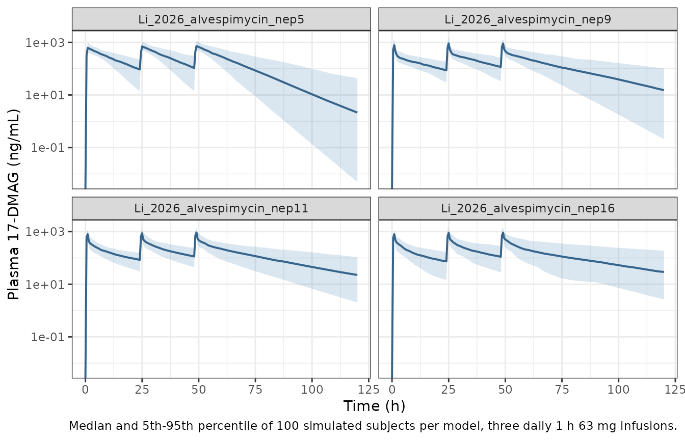
cohortMedians <-
  cohortSim |>
  dplyr::group_by(model) |>
  dplyr::summarise(medCmax = stats::median(Cc[time > 0 & time <= 1.5]),
                   .groups = "drop")

# Cohort-level assertions are made on the centre of the distribution only.
# The extreme of a random cohort is not reproducible across rxode2 builds or
# thread counts (rxSetSeed fixes the draw within a version, not across them).
stopifnot(
  nrow(cohortSim) > 0,
  all(is.finite(cohortSim$Cc)),
  all(cohortSim$Cc >= 0),
  nrow(cohortMedians) == 4L,
  # A 63 mg 1 h infusion into a 29-98 L central volume gives a few hundred
  # ng/mL; this is a wide structural sanity band, not a tuned bound.
  all(cohortMedians$medCmax > 100), all(cohortMedians$medCmax < 3000)
)
PKNCA validation
Non-compartmental analysis of the simulated cohort, one PKNCA run per model over the first dosing interval.
firstInterval <-
  cohortSim |>
  dplyr::filter(time <= 24) |>
  dplyr::mutate(model = as.character(model))

# Defensive time-zero record so PKNCA integrates AUC from the dose time.
firstInterval <-
  dplyr::bind_rows(
    firstInterval,
    firstInterval |>
      dplyr::distinct(model, id) |>
      dplyr::mutate(time = 0, Cc = 0)
  ) |>
  dplyr::distinct(model, id, time, .keep_all = TRUE) |>
  dplyr::arrange(model, id, time)

cohortDose <-
  firstInterval |>
  dplyr::distinct(model, id) |>
  dplyr::mutate(time = 0, amt = 63)

cohortConcObj <- PKNCA::PKNCAconc(firstInterval, Cc ~ time | model + id)
cohortDoseObj <- PKNCA::PKNCAdose(cohortDose, amt ~ time | model + id)
cohortIntervals <- data.frame(
  start = 0, end = 24,
  cmax = TRUE, tmax = TRUE, auclast = TRUE, cav = TRUE
)
cohortNca <- PKNCA::pk.nca(
  PKNCA::PKNCAdata(cohortConcObj, cohortDoseObj, intervals = cohortIntervals)
)

ncaSummary <-
  as.data.frame(cohortNca) |>
  dplyr::filter(PPTESTCD %in% c("cmax", "tmax", "auclast", "cav")) |>
  dplyr::group_by(model, PPTESTCD) |>
  dplyr::summarise(median = stats::median(PPORRES), .groups = "drop") |>
  tidyr::pivot_wider(names_from = PPTESTCD, values_from = median)

ncaSummary |>
  dplyr::rename(
    "Model" = model, "AUC0-24 (ng*h/mL)" = auclast,
    "Cavg (ng/mL)" = cav, "Cmax (ng/mL)" = cmax, "Tmax (h)" = tmax
  ) |>
knitr::kable(digits = 2)| Model | AUC0-24 (ng*h/mL) | Cavg (ng/mL) | Cmax (ng/mL) | Tmax (h) |
|---|---|---|---|---|
| Li_2026_alvespimycin_nep11 | 4652.81 | 193.87 | 828.66 | 1 |
| Li_2026_alvespimycin_nep16 | 4671.17 | 194.63 | 807.97 | 1 |
| Li_2026_alvespimycin_nep5 | 6512.47 | 271.35 | 648.21 | 1 |
| Li_2026_alvespimycin_nep9 | 4587.57 | 191.15 | 838.33 | 1 |
stopifnot(
  nrow(ncaSummary) == 4L,
  all(is.finite(ncaSummary$auclast)),
  # A 1 h infusion peaks at, or immediately after, end of infusion.
  all(ncaSummary$tmax >= 0.5), all(ncaSummary$tmax <= 1.5),
  # Cavg over 0-24 h is AUC0-24 / 24 by construction.
  all(abs(ncaSummary$cav - ncaSummary$auclast / 24) < 1e-6)
)
Comparison against the published parameter values
Li 2026 makes an explicit quantitative claim about these four models in the Results (“Clearance estimates were consistent across the chosen models, ranging from 8.41 to 9.65 L/hr”). The NCA-derived clearance from the typical-value bolus simulation is compared here against the clearance each model reports in Table S2.
publishedCl <- data.frame(
  model  = liModels,
  cl.obs = c(8.41, 9.65, 9.26, 8.64)  # Li 2026 Table S2, models a-d
)
simulatedCl <-
  identityCheck |>
  dplyr::transmute(model, PPTESTCD = "cl.obs", PPORRES = cl_nca)

clTable <- nlmixr2lib::ncaComparisonTable(
  simulated = simulatedCl,
  reference = publishedCl,
  by        = "model",
  units     = c(cl.obs = "L/h")
)
knitr::kable(clTable, digits = 2)| NCA parameter | model | Reference | Simulated | % diff |
|---|---|---|---|---|
| CL/F (L/h) | Li_2026_alvespimycin_nep5 | 8.41 | 8.41 | -0.0% |
| CL/F (L/h) | Li_2026_alvespimycin_nep9 | 9.65 | 9.65 | -0.0% |
| CL/F (L/h) | Li_2026_alvespimycin_nep11 | 9.26 | 9.26 | -0.0% |
| CL/F (L/h) | Li_2026_alvespimycin_nep16 | 8.64 | 8.64 | -0.0% |
attr(clTable, "footnote")
#> NULL
stopifnot(
  # No row exceeds the 20% flagging tolerance.
  !any(grepl("\\*", format(clTable[["% diff"]]))),
  # The paper's stated clearance range across these four models.
  abs(min(publishedCl$cl.obs) - 8.41) < 1e-9,
  abs(max(publishedCl$cl.obs) - 9.65) < 1e-9
)
Cross-check against the stepwise model of the same data set
Aregbe_2012_alvespimycin is the conventional stepwise
three-compartment model of this same 17-DMAG data set. The NSGA-II
three-compartment solutions should land close to it – that is the
“recovers known optimal models” claim of the abstract.
aregbeIni <- rxode2::rxode(readModelDb("Aregbe_2012_alvespimycin"))$iniDf
#> ℹ parameter labels from comments will be replaced by 'label()'
#> Warning: some etas defaulted to non-mu referenced, possible parsing error: etaiov_q_1, etaiov_q_2, etaiov_q_3, etaiov_q_4, etaiov_q_5, etaiov_vc_1, etaiov_vc_2, etaiov_vc_3, etaiov_vc_4, etaiov_vc_5
#> as a work-around try putting the mu-referenced expression on a simple line
aregbeTv  <- function(p) exp(aregbeIni$est[aregbeIni$name == p])

crossCheck <- data.frame(
  Parameter = c("CL (L/h)", "Vc (L)", "Q2 (L/h)", "Vp (L)",
                "Q3 (L/h)", "Vp2 (L)"),
  Aregbe_2012 = c(aregbeTv("lcl"), aregbeTv("lvc"), aregbeTv("lq"),
                  aregbeTv("lvp"), aregbeTv("lq2"), aregbeTv("lvp2")),
  Li_2026_nep11 = c(9.26, 28.1, 81.8, 75.6, 9.47, 85.3),
  Li_2026_nep16 = c(8.64, 29.1, 79.3, 71.9, 9.74, 136)
)
crossCheck$pct_nep16 <-
  100 * (crossCheck$Li_2026_nep16 - crossCheck$Aregbe_2012) /
  crossCheck$Aregbe_2012
crossCheck |>
  dplyr::rename(
    "Aregbe 2012 (stepwise)" = Aregbe_2012,
    "Li 2026, NEP = 11" = Li_2026_nep11,
    "Li 2026, NEP = 16" = Li_2026_nep16,
    "% diff (NEP 16 vs stepwise)" = pct_nep16
  ) |>
knitr::kable(digits = 2)| Parameter | Aregbe 2012 (stepwise) | Li 2026, NEP = 11 | Li 2026, NEP = 16 | % diff (NEP 16 vs stepwise) |
|---|---|---|---|---|
| CL (L/h) | 8.4 | 9.26 | 8.64 | 2.86 |
| Vc (L) | 27.4 | 28.10 | 29.10 | 6.20 |
| Q2 (L/h) | 85.1 | 81.80 | 79.30 | -6.82 |
| Vp (L) | 66.4 | 75.60 | 71.90 | 8.28 |
| Q3 (L/h) | 11.6 | 9.47 | 9.74 | -16.03 |
| Vp2 (L) | 142.0 | 85.30 | 136.00 | -4.23 |
stopifnot(
  # Clearance and the fast-distribution parameters agree closely between the
  # stepwise and machine-search three-compartment fits of the same data.
  abs(crossCheck$pct_nep16[crossCheck$Parameter == "CL (L/h)"]) < 10,
  abs(crossCheck$pct_nep16[crossCheck$Parameter == "Q2 (L/h)"]) < 10,
  abs(crossCheck$pct_nep16[crossCheck$Parameter == "Q3 (L/h)"]) < 20
)
Every parameter of the NEP = 16 machine-search solution lands within
about 16% of the stepwise fit, which is a strong independent check on
the transcription: two different search procedures applied to the same
951 concentrations arrive at essentially the same three-compartment
system. The one parameter that does move materially across the Pareto
front is the deep peripheral volume Vp2 (85.3 L at NEP = 11
against 136 L at NEP = 16 and 142 L stepwise) – expected, since it is
the least well identified parameter in a three-compartment model of a
102 h sampling window, and Li 2026 itself notes the higher uncertainty
on the volume terms of the more complex non-dominated solutions.
Assumptions and deviations
Errata and interpretation of the source
The
Q2/Q3variability rows of Table S2 are transposed. In Li 2026 Supplementary Table S2, model d, the 75.8% between-subject and 28.6% between-occasion terms are both printed on theQ3row, leavingQ2with no variability. Three independent sources say otherwise: Li 2026’s own Table S3 lists the model dBOVset asV, CL, Q2; the parameter table of Li 2024 for this identical model puts 28.6% onQ2and 75.8% onQ3; and the deposited final control stream definesIOVQ2acting onQ2while writingQ3 = THETA(4)*EXP(ETA(12)).Li_2026_alvespimycin_nep16follows the control stream: BOV onQ2, BSV onQ3.The residual-error column of Table S2 reports NONMEM
$SIGMAvariances, not standard deviations. Two checks fix this. First, the residual reported for model d (0.017) has a square root of 0.130, and Li 2024 reports “13.2” for the proportional error of this identical model – so the 2026 table reports the variance where the 2024 table reports the percent SD. Second, the relative standard error attached to these entries (6-7%) is about twice the 2.7% that Aregbe 2012 reports for the SD of the proportional error on the same data, which is the expected doubling when the reported quantity is a variance rather than an SD. All four model files therefore take the square root of the tabulated value.Concentrations were modelled on the ng/mL scale, despite the “(mg/L)” label on the additive-error row. The deposited control stream sets
S1 = V1with no scaling factor, so the concentration scale is fixed by the units of the data set’sAMTcolumn, which the control stream does not state. Two pieces of evidence resolve it to ng/mL: the pcVPC concentration axes of Li 2026 Figure 2 run to roughly 2500, which is the ng/mL magnitude for this drug and dose range and is three orders of magnitude away from the mg/L magnitude; and the$SIGMAinitial estimate for the additive term is 1, which is a sensible assay-noise starting value in ng/mL and an absurd one in mg/L. The model files therefore writeCc = 1000 * central / vc, taking doses in mg and returning ng/mL, andaddSdis expressed in ng/mL.The
propresidual token is exponential, not proportional. Li 2026 Table S3 labels the residual model of the four packaged modelsprop,prop,propandcomb, but the deposited token file writes both asIOBS = F*EXP(EPS(1))andIOBS = F*EXP(EPS(1)) + EPS(2). That is a log-normal residual. Models a, b and c are encoded faithfully asCc ~ lnorm(expSd). Model d cannot be:rxode2parses anlnorm() + add()endpoint but cannot solve it (cannot find additive standard deviation for 'Cc'), so model d is encoded asCc ~ prop(propSd) + add(addSd). The two forms agree to second order at this residual magnitude (exp(0.130) - 1 = 0.139).The weight centring constant is not in Li 2026. Table S2 reports the power exponent 1.31 but never states what weight it is centred on. The value 81 kg is read from the deposited pyDarwin template and final control stream for this same search space (
CWTKGONE = WT/81 ;; WEIGHT CENTERED ON ONE). Note this is close to but not identical with the cohort median of 80.3 kg reported in Table S1; the constant is a round number chosen by the authors, not the cohort median.The unit on the dose column of Table 1 is inconsistent with the source study. Li 2026 Table 1 reports the DMAG dose as “33 mg (2.2-413 mg)”. Aregbe 2012, the stepwise analysis of this same data set, reports the same two extremes as 2.2-413 mg/m^2. The model files record Li 2026’s numbers as printed and flag the discrepancy; the simulations in this vignette use 63 mg, which is the Table 1 median scaled by a 1.9 m^2 body surface area, and no packaged parameter depends on the choice.
The demographic split differs between the two papers. Li 2026 Table S1 reports the DMAG cohort as 41 (62%) male and 25 (38%) female; Li 2024 states “39% (26 of 66) male and 61% (40 of 66) female” for the same 66 subjects. The model files follow Li 2026, the paper being extracted. Sex is not a retained covariate in any of the four packaged models, so nothing in the models depends on this.
The occasion count is three. Neither the number of occasions nor the occasion definition appears in Li 2026. The deposited control stream writes the between-occasion blocks for
OCCvalues 1, 2 and 3 only, so three occasions are carried. Aregbe 2012’s analysis of the same data set uses up to five daily dosing occasions; users applying these models to a data set with more than three occasions will need to extend theoc*indicator set.
Assumptions made because the source is silent
SEXreference level. The pyDarwin token file offers*EXP(THETA(...)*SEX)effects onVcandCL, but neither publication states whether the data set’sSEXcolumn codes 1 for male or for female. Since no packaged model retains a sex effect, this is recorded incovariatesDataExcludedrather than resolved.Weight distribution of the virtual cohort. Table S1 reports the median and range of weight but not its shape. A log-normal draw truncated to the reported range is used here; it affects only the virtual cohort figure, not any packaged parameter.
No observed data. The 17-DMAG concentrations are not redistributed with this package, so the pcVPCs of Li 2026 Figure 2 cannot be reproduced directly. The structural consequence the figure illustrates – the progressive change in the shape of the predicted profile from one to three compartments – is checked instead.
Convention deviations
covariatesDataExcludedis used in all four files to record the covariates the search space screened but the packaged solutions did not retain. This is documentation only and is not referenced inmodel().Model d encodes the multiplicative residual as
prop()rather than the source’s exponential form, for the solver reason given above. Models a, b and c uselnorm(), so the residual-error family is deliberately not uniform across the four sibling files.