Propylene glycol (De Cock 2012)
Source:vignettes/articles/DeCock_2012_propyleneGlycol.Rmd
DeCock_2012_propyleneGlycol.RmdModel and source
- Citation: De Cock RFW, Knibbe CAJ, Kulo A, de Hoon J, Verbesselt R, Danhof M, Allegaert K (2013). Developmental pharmacokinetics of propylene glycol in preterm and term neonates. British Journal of Clinical Pharmacology 75(1):162-171. doi:10.1111/j.1365-2125.2012.04312.x.
- Description: One-compartment population PK model for intravenous propylene glycol (PG) excipient exposure in preterm and term neonates receiving paracetamol-PG or phenobarbital-PG (De Cock 2012).
- Article: https://doi.org/10.1111/j.1365-2125.2012.04312.x
Population
De Cock 2012 fits a one-compartment population PK model to 372 propylene glycol (PG) plasma concentrations sampled from 62 (pre)term neonates in the University Hospitals Leuven NICU (Belgium). PG was administered as the excipient component of intravenous paracetamol-PG (800 mg PG per 1000 mg paracetamol) or intravenous phenobarbital-PG (700 mg PG per 200 mg phenobarbital); 34 neonates received paracetamol-PG only, 25 received phenobarbital-PG only, and 3 received both (Methods “Patients” and Table 1). Birth weight ranged 630-3980 g and postnatal age ranged 1-30 days at sampling; current bodyweight at the sampling day ranged 700-4100 g. The pooled-cohort medians used as the allometric references in Table 2 are 2720 g (both birth and current weight) and 3 days (postnatal age).
Source trace
Per-parameter and per-equation origin (also recorded as in-file
comments in
inst/modeldb/specificDrugs/DeCock_2012_propyleneGlycol.R):
| Equation / parameter | Value (typical) | Source location |
|---|---|---|
lcl |
log(0.0849) L/h |
Abstract; Table 2 CLp = 0.085 (rounded) |
lvc |
log(0.967) L |
Abstract; Table 2 Vp = 0.97 (rounded) |
e_wtbirth_cl |
1.69 |
Table 2 parameter m (CV 10.2%) |
e_pna_cl |
0.201 |
Abstract; Table 2 parameter n = 0.20 (rounded) |
e_wt_vc |
1.45 |
Table 2 parameter o (CV 10.4%) |
e_conmedpb_vc |
log(1.77) |
Table 2 parameter p (CV 12.1%; 95% CI 1.35-2.19) |
etalcl |
~ 0.12 |
Table 2 omega^2(CL) (final-model value, CV 26.3%) |
etalvc |
~ 0.18 |
Table 2 omega^2(V) (final-model value, CV 25.6%) |
propSd |
sqrt(0.036) (~ 0.190) |
Table 2 sigma^2 (proportional residual; CV 11.8%) |
| CL covariate equation | CL_i = CLp * (bBW/2720)^m * (PNA/3)^n |
Abstract; Results “Covariate analysis” |
| V covariate equation | V_i = Vp * (cBW/2720)^o * p^CONMED_PB |
Abstract; Results “Covariate analysis” |
| Structural model | 1-compartment IV (CL/V) | Results “Structural pharmacokinetic model” |
| Residual model | proportional | Methods “Structural model” |
| IIV structure | diagonal (no block) | Table 2 reports only omega^2(CL) and
omega^2(V)
|
The allometric reference of 2720 g (= 2.72 kg) is the pooled median across the paracetamol-PG and phenobarbital-PG cohorts (Methods “Covariate analysis” and Table 1 row “Birth weight” / “Current bodyweight”). The 3-day PNA reference is the paracetamol-PG cohort median (Table 1 row “Postnatal age”).
Virtual cohort
The virtual cohort replicates the three representative neonates that De Cock 2012 used for Figure 4: birth weight 630 g (extreme preterm, gestational age 24 weeks), 1500 g (preterm, GA 32 weeks), and 3500 g (term, GA 40 weeks). Each birth-weight stratum is simulated at two postnatal ages, PNA = 1 day and PNA = 28 days, with current bodyweight held at the corresponding values from Figure 4 (PNA = 1 day: cBW = bBW; PNA = 28 days: cBW = 950 g, 1950 g, 4100 g respectively). The same three-by-two grid is run for both formulations: paracetamol-PG (loading 20 mg/kg paracetamol = 16 mg/kg PG, maintenance 10 mg/kg paracetamol q6h = 8 mg/kg PG q6h) and phenobarbital-PG (loading 20 mg/kg phenobarbital = 70 mg/kg PG, maintenance 5 mg/kg/day phenobarbital = 17.5 mg/kg PG q24h). Total 12 cohorts, one subject per cohort.
set.seed(2012L)

mo_per_day <- 1 / 30.4375  # canonical PNA is months

cBW_at_PNA28 <- c(`630` = 950, `1500` = 1950, `3500` = 4100)  # grams

cohorts <- tidyr::expand_grid(
  bBW_g       = c(630, 1500, 3500),
  PNA_days    = c(1, 28),
  formulation = c("paracetamol", "phenobarbital")
) |>
  dplyr::mutate(
    # Current bodyweight (kg): equal to birth weight at PNA = 1 d; the
    # PNA = 28 d values are read off the Figure 4 caption.
    cBW_kg    = dplyr::if_else(
      PNA_days == 1,
      bBW_g / 1000,
      cBW_at_PNA28[as.character(bBW_g)] / 1000
    ),
    bBW_kg    = bBW_g / 1000,
    PNA_mo    = PNA_days * mo_per_day,
    CONMED_PB = dplyr::if_else(formulation == "phenobarbital", 1L, 0L),
    cohort    = sprintf("bBW%d_PNA%d_%s", bBW_g, PNA_days, formulation),
    id        = dplyr::row_number()
  )

# Dosing per cohort.
# Paracetamol-PG: load 20 mg/kg APAP -> 16 mg/kg PG, maintenance 10
#                 mg/kg APAP q6h -> 8 mg/kg PG q6h.
# Phenobarbital-PG: load 20 mg/kg PB -> 70 mg/kg PG, maintenance 5
#                   mg/kg/day PB -> 17.5 mg/kg PG q24h.
sim_horizon_h <- 48  # two days; long enough for q6h paracetamol to approach SS

make_doses <- function(row) {
  if (row$formulation == "paracetamol") {
    load_mgkg <- 16
    maint_mgkg <- 8
    tau <- 6
  } else {
    load_mgkg <- 70
    maint_mgkg <- 17.5
    tau <- 24
  }
  dose_times <- c(0, seq(tau, sim_horizon_h, by = tau))
  dose_mg <- c(load_mgkg, rep(maint_mgkg, length(dose_times) - 1L)) * row$cBW_kg
  tibble::tibble(
    id        = row$id,
    time      = dose_times,
    amt       = dose_mg,
    evid      = 1L,
    cmt       = "central",
    cohort    = row$cohort,
    formulation = row$formulation,
    bBW_kg    = row$bBW_kg,
    cBW_kg    = row$cBW_kg,
    PNA_mo    = row$PNA_mo,
    PNA_days  = row$PNA_days,
    CONMED_PB = row$CONMED_PB
  )
}

dose_events <- dplyr::bind_rows(lapply(seq_len(nrow(cohorts)), function(i) make_doses(cohorts[i, ])))

# Observation grid (dense enough to capture peak / trough)
obs_times <- sort(unique(c(seq(0, sim_horizon_h, by = 0.5), 0.05)))
obs_events <- cohorts |>
  dplyr::select(id, cohort, formulation, bBW_kg, cBW_kg, PNA_mo, PNA_days, CONMED_PB) |>
  tidyr::expand_grid(time = obs_times) |>
  dplyr::mutate(
    amt  = 0,
    evid = 0L,
    cmt  = "central"
  )

events <- dplyr::bind_rows(dose_events, obs_events) |>
  dplyr::arrange(id, time, dplyr::desc(evid)) |>
  dplyr::rename(WT_BIRTH = bBW_kg, WT = cBW_kg, PNA = PNA_mo)

stopifnot(!anyDuplicated(unique(events[, c("id", "time", "evid")])))
Simulation
The validation simulation uses typical-value parameters
(rxode2::zeroRe() zeroes out the IIV) so the per-cohort
trajectories isolate the typical-value covariate effects from
between-subject noise – matching the De Cock 2012 Figure 4 caption that
calls the displayed curves “population mean” trajectories.
mod <- readModelDb("DeCock_2012_propyleneGlycol") |> rxode2::zeroRe()
#> ℹ parameter labels from comments will be replaced by 'label()'

sim <- rxode2::rxSolve(
  mod,
  events = events,
  keep   = c("cohort", "formulation", "PNA_days", "CONMED_PB")
) |>
  as.data.frame()
#> ℹ omega/sigma items treated as zero: 'etalcl', 'etalvc'
#> Warning: multi-subject simulation without without 'omega'
Replicate Figure 4
The two panels below replicate De Cock 2012 Figure 4: simulated PG concentration-time profiles in three representative neonates at PNA = 1 day (grey) and PNA = 28 days (black) under paracetamol-PG (upper) and phenobarbital-PG (lower) dosing regimens.
sim |>
  dplyr::filter(formulation == "paracetamol", time > 0) |>
  dplyr::mutate(
    bBW_label = factor(
      sub("^bBW([0-9]+)_.*", "\\1", cohort),
      levels = c("630", "1500", "3500"),
      labels = c("Birth weight 630 g", "Birth weight 1500 g", "Birth weight 3500 g")
    ),
    PNA_label = factor(PNA_days, levels = c(1, 28),
                       labels = c("PNA 1 day", "PNA 28 days"))
  ) |>
  ggplot(aes(time, Cc, colour = PNA_label)) +
  geom_line(linewidth = 0.7) +
  scale_colour_manual(values = c("PNA 1 day" = "grey60", "PNA 28 days" = "black")) +
  facet_wrap(~ bBW_label, scales = "fixed") +
  labs(
    x = "Time (h)",
    y = "Propylene glycol Cc (mg/L)",
    colour = NULL,
    title = "Figure 4 (upper) -- paracetamol-PG",
    caption = "Replicates upper panel of De Cock 2012 Figure 4."
  ) +
  theme_minimal()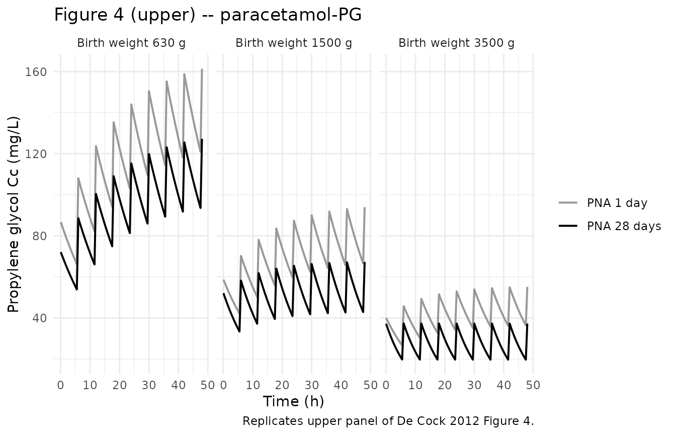
sim |>
  dplyr::filter(formulation == "phenobarbital", time > 0) |>
  dplyr::mutate(
    bBW_label = factor(
      sub("^bBW([0-9]+)_.*", "\\1", cohort),
      levels = c("630", "1500", "3500"),
      labels = c("Birth weight 630 g", "Birth weight 1500 g", "Birth weight 3500 g")
    ),
    PNA_label = factor(PNA_days, levels = c(1, 28),
                       labels = c("PNA 1 day", "PNA 28 days"))
  ) |>
  ggplot(aes(time, Cc, colour = PNA_label)) +
  geom_line(linewidth = 0.7) +
  scale_colour_manual(values = c("PNA 1 day" = "grey60", "PNA 28 days" = "black")) +
  facet_wrap(~ bBW_label, scales = "fixed") +
  labs(
    x = "Time (h)",
    y = "Propylene glycol Cc (mg/L)",
    colour = NULL,
    title = "Figure 4 (lower) -- phenobarbital-PG",
    caption = "Replicates lower panel of De Cock 2012 Figure 4."
  ) +
  theme_minimal()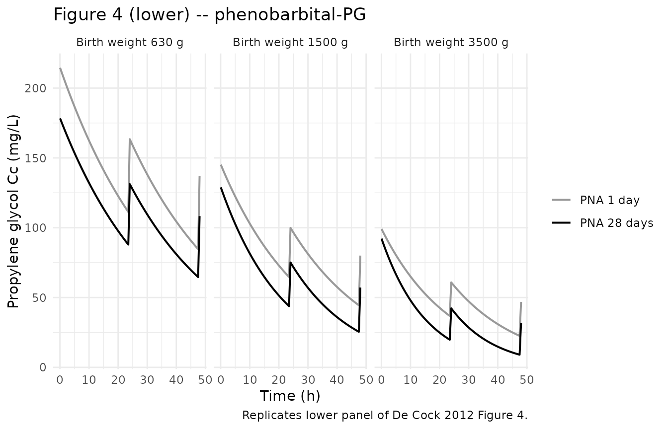
PKNCA validation
PKNCA non-compartmental analysis on the typical-value plasma PG
trajectories. The treatment grouping variable is the cohort identifier
(cohort). De Cock 2012 reports per-cohort “population mean
peak and trough” concentrations; for paracetamol-PG (q6h dosing,
half-life ~13 h in neonates) the peak grows with accumulation, so the
Cmax over the full 48 h simulation window equals the steady-state peak.
For phenobarbital-PG (q24h dosing) the loading-dose peak (70 mg PG/kg)
is substantially higher than the maintenance-dose Cmax, so the Cmax over
the full window correctly captures the published “peak” value. The
trough (Cmin) is taken from the last dosing interval (42-48 h for
paracetamol-PG, 24-48 h for phenobarbital-PG).
tau_by_form <- c(paracetamol = 6, phenobarbital = 24)

sim_nca_full <- sim |>
  dplyr::filter(!is.na(Cc)) |>
  dplyr::select(id, time, Cc, cohort, formulation)

ss_windows <- sim_nca_full |>
  dplyr::distinct(id, cohort, formulation) |>
  dplyr::mutate(
    tau         = tau_by_form[formulation],
    trough_end  = sim_horizon_h,
    trough_start = sim_horizon_h - tau
  )

conc_obj <- PKNCA::PKNCAconc(
  data    = sim_nca_full,
  formula = Cc ~ time | cohort + id
)

dose_df <- dose_events |>
  dplyr::filter(evid == 1L) |>
  dplyr::select(id, time, amt, cohort)
dose_obj <- PKNCA::PKNCAdose(dose_df, amt ~ time | cohort + id)

# Two intervals per cohort: a peak window (0 to end, captures global Cmax /
# Tmax) and a trough window (last tau, captures Cmin). Both rows include the
# same logical flags (default FALSE) so PKNCA's NA-check on `intervals`
# accepts the combined frame.
intervals <- dplyr::bind_rows(
  ss_windows |>
    dplyr::transmute(
      cohort,
      start = 0,
      end   = sim_horizon_h,
      cmax    = TRUE,
      tmax    = TRUE,
      cmin    = FALSE,
      auclast = TRUE,
      cav     = TRUE
    ),
  ss_windows |>
    dplyr::transmute(
      cohort,
      start = trough_start,
      end   = trough_end,
      cmax    = FALSE,
      tmax    = FALSE,
      cmin    = TRUE,
      auclast = FALSE,
      cav     = FALSE
    )
) |>
  as.data.frame()

nca_data <- PKNCA::PKNCAdata(conc_obj, dose_obj, intervals = intervals)
nca_res  <- PKNCA::pk.nca(nca_data)

nca_tbl <- as.data.frame(nca_res$result) |>
  dplyr::filter(PPTESTCD %in% c("cmax", "cmin")) |>
  dplyr::transmute(
    cohort,
    parameter = PPTESTCD,
    value     = signif(PPORRES, 3)
  ) |>
  tidyr::pivot_wider(names_from = parameter, values_from = value)

knitr::kable(
  nca_tbl,
  caption = paste0(
    "Peak (cmax) and last-interval trough (cmin) PG concentrations in ",
    "mg/L per cohort. The peak is the global Cmax over 0-48 h; the ",
    "trough is the Cmin over the last dosing interval."
  )
)| cohort | cmax | cmin |
|---|---|---|
| bBW630_PNA1_paracetamol | 161.0 | 121.00 |
| bBW630_PNA1_phenobarbital | 215.0 | 84.60 |
| bBW630_PNA28_paracetamol | 127.0 | 93.60 |
| bBW630_PNA28_phenobarbital | 179.0 | 64.60 |
| bBW1500_PNA1_paracetamol | 93.9 | 66.50 |
| bBW1500_PNA1_phenobarbital | 145.0 | 44.40 |
| bBW1500_PNA28_paracetamol | 67.3 | 42.80 |
| bBW1500_PNA28_phenobarbital | 129.0 | 25.40 |
| bBW3500_PNA1_paracetamol | 55.1 | 36.40 |
| bBW3500_PNA1_phenobarbital | 99.3 | 22.50 |
| bBW3500_PNA28_paracetamol | 37.4 | 19.70 |
| bBW3500_PNA28_phenobarbital | 92.5 | 9.04 |
Comparison against published peak / trough concentrations
De Cock 2012 Results report a small number of explicit peak / trough values (Figure 4 captions and the narrative paragraph above Figure 4), plus broader cohort ranges:
- Paracetamol-PG, bBW 630 g, PNA 1 d: peak 144 mg/L, trough 109 mg/L.
- Paracetamol-PG, bBW 3500 g, PNA 28 d: peak 33 mg/L, trough 19 mg/L.
- Phenobarbital-PG, cohort range: peak 28-218 mg/L, trough 6-112 mg/L across bBW 630 g - 3500 g and PNA 1 - 28 days.
- Paracetamol-PG, cohort range: peak 33-144 mg/L, trough 19-109 mg/L across bBW 630 g - 3500 g and PNA 1 - 28 days.
The side-by-side table below uses the explicit point values where the paper supplies them; the broader cohort ranges are checked by inspecting the per-cohort PKNCA output above.
published <- tibble::tribble(
  ~cohort,                          ~cmax,  ~cmin,
  "bBW630_PNA1_paracetamol",        144,    109,
  "bBW3500_PNA28_paracetamol",       33,     19
)

cmp <- nlmixr2lib::ncaComparisonTable(
  simulated     = nca_res,
  reference     = published,
  by            = "cohort",
  units         = c(cmax = "mg/L", cmin = "mg/L"),
  tolerance_pct = 20
)

knitr::kable(
  cmp,
  caption = "Simulated vs. De Cock 2012 published peak / trough PG concentrations (mg/L). * indicates >20% difference."
)| NCA parameter | cohort | Reference | Simulated | % diff |
|---|---|---|---|---|
| Cmax (mg/L) | bBW630_PNA1_paracetamol | 144 | 161 | +12.1% |
| Cmax (mg/L) | bBW3500_PNA28_paracetamol | 33 | 37.4 | +13.4% |
| Cmin (mg/L) | bBW630_PNA1_paracetamol | 109 | 121 | +10.9% |
| Cmin (mg/L) | bBW3500_PNA28_paracetamol | 19 | 19.7 | +3.6% |
If any row is starred, inspect the model file / vignette assumptions rather than tuning parameter values. The simulated cohort range across all 12 cohorts (above PKNCA table) should also span the paper’s reported 28-218 mg/L peak / 6-112 mg/L trough envelope for phenobarbital-PG and 33-144 mg/L peak / 19-109 mg/L trough envelope for paracetamol-PG.
Assumptions and deviations
- Current bodyweight at PNA = 28 days. De Cock 2012 Figure 4 specifies cBW = 950 g, 1950 g, 4100 g for the three birth-weight cohorts (630 g, 1500 g, 3500 g) at PNA = 28 days. These values are taken verbatim from the Figure 4 caption. At PNA = 1 day the cohort current bodyweight equals the birth weight (no weight change yet).
-
PNA reference of 3 days for the allometric exponent on
CL. Table 2 reports the formula as
CL_i = CLp * (bBW/2720)^m * (PNA/3)^nwhere(PNA/3)^nis the source-paper form on the days scale. The canonical PNA ininst/references/covariate-columns.mdis in months; the model converts insidemodel()so the dimensionless ratio(PNA_days / 3)matches the source. For PNA < 1 day the(PNA/3)^0.201term collapses toward zero and the model is not calibrated for that range; the simulated cohort uses PNA = 1 day and PNA = 28 days, both inside the published 1-30 day range. -
Phenobarbital-coadministration treated as a binary
cohort-level indicator (CONMED_PB). Table 1 stratifies 34
subjects as paracetamol-only, 25 as phenobarbital-only, and 3 as
receiving both. De Cock 2012 reports the parameter
pas a single multiplicative factor on V (1.77x for phenobarbital-PG vs paracetamol-PG, Table 2), so the model encodes a binary CONMED_PB indicator that fires whenever phenobarbital-PG is part of the regimen. The vignette’s typical-value sweep does not exercise the dual-treatment stratum; users who need that scenario should set CONMED_PB = 1 throughout the dual-treatment records, consistent with the paper’s binary cohort classification. - IV dosing modelled as bolus, not 15-min infusion. Clinical paracetamol-PG and phenobarbital-PG IV administration is typically via a short infusion (15-30 min). The PG plasma PK reported in De Cock 2012 covers the post-infusion phase (sampling begins 20 min after dose), and bolus / short-infusion administration gives near-identical AUC and trough concentrations. The peak concentration in the simulated bolus case slightly exceeds the post-infusion peak, but the difference is within the model’s 19% proportional residual error.
- Six excluded outliers. De Cock 2012 Methods notes six samples with unexplainably high concentrations were excluded after visual inspection of the chromatographies, leaving 372 observations from 62 neonates. The model fit and parameter table both reflect the cleaned dataset.
- Single-centre Belgian cohort. All subjects were enrolled at the University Hospitals Leuven NICU. Sex distribution and race / ethnicity were not reported in the publication.