RBP-7000 (Ivaturi 2017)
Source:vignettes/articles/Ivaturi_2017_RBP_7000.Rmd
Ivaturi_2017_RBP_7000.RmdModel and source
- Citation: Ivaturi V, Gopalakrishnan M, Gobburu JVS, Zhang W, Liu Y, Heidbreder C, Laffont CM (2017). Exposure-response analysis after subcutaneous administration of RBP-7000, a once-a-month long-acting Atrigel formulation of risperidone. British Journal of Clinical Pharmacology 83(7):1476-1498. doi:10.1111/bcp.13246
- Article: Br J Clin Pharmacol 83(7):1476-1498
RBP-7000 is a once-monthly long-acting subcutaneous (SC) ATRIGEL formulation of risperidone developed by Indivior for the treatment of schizophrenia. Ivaturi 2017 reports the integrated population PK / PANSS PD analysis of a Phase 3 registration trial (NCT02109562) where 337 adults with acute schizophrenia received two SC injections of RBP-7000 (90 mg or 120 mg) or placebo 28 days apart over an 8-week double-blind period. The PK sub-model is the empirical dual-absorption structure inherited from the upstream RBP-7000 SAD / MAD studies (Gomeni 2013; Laffont 2014, 2015) and re-estimated against the sparse Phase 3 PK design. The PD sub-model relates total active moiety plasma concentrations (risperidone + 9-OH-risperidone, molecular-weight corrected) to PANSS total scores via a Weibull placebo response and an Emax drug effect.
Population
The 337 ITT subjects (placebo n = 112; 90 mg n = 111; 120 mg n = 114) had a mean age of 41-43 years across treatment arms, mean body weight 88-93 kg, mean body-mass index 29-31 kg/m^2, and were 73-84% male. The cohort was 70-75% Black or African-American and 91-94% non-Hispanic / non-Latino (Table 1). All subjects had a screening PANSS total score 80-120 with at least two of four positive subscale items scoring >4 (Methods). CYP2D6 phenotype distribution across arms: 82-88% extensive metabolizers, 3.6-7.1% intermediate, 0.9-2.6% poor, and 5.2-7.1% inconclusive (Table 1).
The full population metadata are available programmatically via
modellib() (the model’s row in the modeldb data frame; the
description and per-cohort metadata are embedded in the
model file under
inst/modeldb/specificDrugs/Ivaturi_2017_RBP_7000.R).
Source trace
The per-parameter origin is recorded as an in-file comment next to
each ini() entry in
inst/modeldb/specificDrugs/Ivaturi_2017_RBP_7000.R. The
table below collects them in one place for review.
| Equation / parameter | Value | Source location |
|---|---|---|
lka1 (fast first-order abs) |
log(0.005) | Table 2 / A2: ka1 = 0.005 1/h |
lka2 (slow abs from transit5) |
log(0.016) | Table 2 / A2: ka2 = 0.016 1/h |
lktr (transit rate) |
log(0.023) | Table 2 / A2: ktr = 0.023 1/h |
lkel (risperidone elim) |
log(0.043) | Table A2 (Phase-3): krel = 0.043 1/h |
lkmet (metabolite formation) |
log(0.221) | Table A2 (Phase-3): kr9 = 0.221 1/h |
lkel_9oh (9-OH elim) |
log(0.069) | Table A2 (Phase-3): k9el = 0.069 1/h |
lk12 (central to peripheral) |
log(0.841) | Table A2 (Phase-3): krrp = 0.841 1/h |
lk21 (peripheral to central) |
log(0.006) | Table A2 (Phase-3): krpr = 0.006 1/h |
lvc (apparent central volume) |
log(129) | Table A2 (Phase-3): V = 129 L |
e_cyp2d6_im_kmet (IM on kr9) |
-0.76 | Table 2: CYP2D6 Intermediate effect on metabolite formation |
e_cyp2d6_pm_kmet (PM on kr9) |
-0.94 | Table 2: CYP2D6 Poor effect on metabolite formation |
| PK ODE structure (depot / 5 transit / 2-cmt central / 9-OH) | n/a | Figure 1 and Pharmacokinetic model section |
| Total active moiety formula | (410/426) | Pharmacodynamic model for PANSS section:
[AM] = [risperidone] + [9-OH-risperidone] * (410/426)
|
bsl (baseline PANSS) |
94.9 | Table 3 exposure-response model |
pmax, tprog, pow
|
0.06, 1.7 wk, 2.1 | Table 3 exposure-response model |
drift (linear drift) |
-1.2 PANSS/wk | Table 3 exposure-response model |
emax, ec50
|
0.054, 4.6 ng/mL | Table 3 exposure-response model |
| PANSS PD equation | n/a | Figure 1 box; Results ‘PK/PD analysis for PANSS score’ |
| Residual error (combined add+prop) | propSd 0.297, addSd 0.137 ng/mL | Table A2 (Phase-3); shared between risperidone and 9-OH-risperidone |
| PANSS residual error (additive) | 5.5 PANSS units | Table 3 exposure-response model |
Virtual cohort
Original observed data are not publicly available. The figures below use a typical-value individual at the cohort median to reproduce the published mean concentration-time profiles (Figure 2) and PANSS trajectory (Figure 4). The cohort is a CYP2D6 extensive metabolizer (the most common phenotype in the trial, 82-88% of subjects across arms).
mod_fn      <- readModelDb("Ivaturi_2017_RBP_7000")
mod         <- rxode2::rxode2(mod_fn())
mod_typical <- rxode2::zeroRe(mod)

# Two-injection 8-week regimen: 90 mg or 120 mg SC at t = 0 and t = 28 days,
# sampled hourly over the 57-day study window. Both arms use the EM /
# Inconclusive reference (CYP2D6_PM = 0 and CYP2D6_IM = 0).
treatment_grid <- tibble::tibble(
  treatment = c("90 mg", "120 mg"),
  dose_mg   = c(90, 120)
)

make_events <- function(dose_mg, treatment) {
  hour_grid <- seq(0, 57 * 24, by = 6)
  ev <- rxode2::et(amt = dose_mg, time = 0,       cmt = "depot")
  ev <- rxode2::et(ev, amt = dose_mg, time = 28 * 24, cmt = "depot")
  ev <- rxode2::et(ev, hour_grid, cmt = "Cc")
  out <- as.data.frame(ev)
  out$CYP2D6_PM <- 0
  out$CYP2D6_IM <- 0
  out$treatment <- treatment
  out
}

events <- dplyr::bind_rows(lapply(seq_len(nrow(treatment_grid)), function(i) {
  make_events(treatment_grid$dose_mg[i], treatment_grid$treatment[i])
}))
events$id <- match(events$treatment, treatment_grid$treatment)
Simulation
sim <- rxode2::rxSolve(
  mod_typical,
  events     = events,
  keep       = c("treatment"),
  returnType = "data.frame"
)
#> ℹ omega/sigma items treated as zero: 'etalka1', 'etalka2', 'etalktr', 'etalkmet', 'etalkel_9oh', 'etalk12', 'etalk21', 'etalvc', 'etabsl', 'etapmax', 'etadrift'
#> Warning: multi-subject simulation without without 'omega'
sim$time_day <- sim$time / 24
Replicate published figures
Figure 2 – concentration-time profiles by dose
sim |>
  dplyr::filter(time_day > 0) |>
  dplyr::select(time_day, treatment, Risperidone = Cc, `9-OH-Risperidone` = Cc_9oh) |>
  tidyr::pivot_longer(c(Risperidone, `9-OH-Risperidone`), names_to = "analyte", values_to = "conc") |>
  ggplot(aes(time_day, conc, colour = treatment)) +
  geom_line(linewidth = 0.7) +
  facet_wrap(~analyte, scales = "free_y") +
  scale_x_continuous(breaks = c(1, 8, 15, 22, 29, 36, 43, 50, 57)) +
  labs(x = "Days after first dose",
       y = "Plasma concentration (ng/mL)",
       colour = "Dose")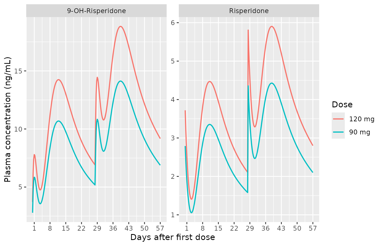
Replicates Figure 2 of Ivaturi 2017: mean risperidone and 9-OH-risperidone plasma concentration-time profiles for the 90 mg and 120 mg RBP-7000 arms. Concentrations are plotted from 1 day post-dose (matching the paper’s sampling windows: Days 1-3, 8-15, 16-22, pre-Day-29, 29-31, 36-42, 43-49, 55-57).
Figure 4 – PANSS trajectory by dose
# Sham 0 mg events for the placebo arm -- same structure, dose_mg = 0 so AM is
# zero and only the Weibull placebo response + linear drift drives PANSS.
ev_placebo <- make_events(0, "Placebo")
ev_placebo$id <- 0L
ev_all <- dplyr::bind_rows(events, ev_placebo)
sim_panss <- rxode2::rxSolve(
  mod_typical,
  events     = ev_all,
  keep       = c("treatment"),
  returnType = "data.frame"
)
#> ℹ omega/sigma items treated as zero: 'etalka1', 'etalka2', 'etalktr', 'etalkmet', 'etalkel_9oh', 'etalk12', 'etalk21', 'etalvc', 'etabsl', 'etapmax', 'etadrift'
#> Warning: multi-subject simulation without without 'omega'
sim_panss$time_day <- sim_panss$time / 24

sim_panss |>
  dplyr::filter(time_day >= 0) |>
  ggplot(aes(time_day, PANSS, colour = treatment)) +
  geom_line(linewidth = 0.7) +
  scale_x_continuous(breaks = c(0, 14, 28, 42, 56)) +
  labs(x = "Days after first dose",
       y = "PANSS total score",
       colour = "Arm")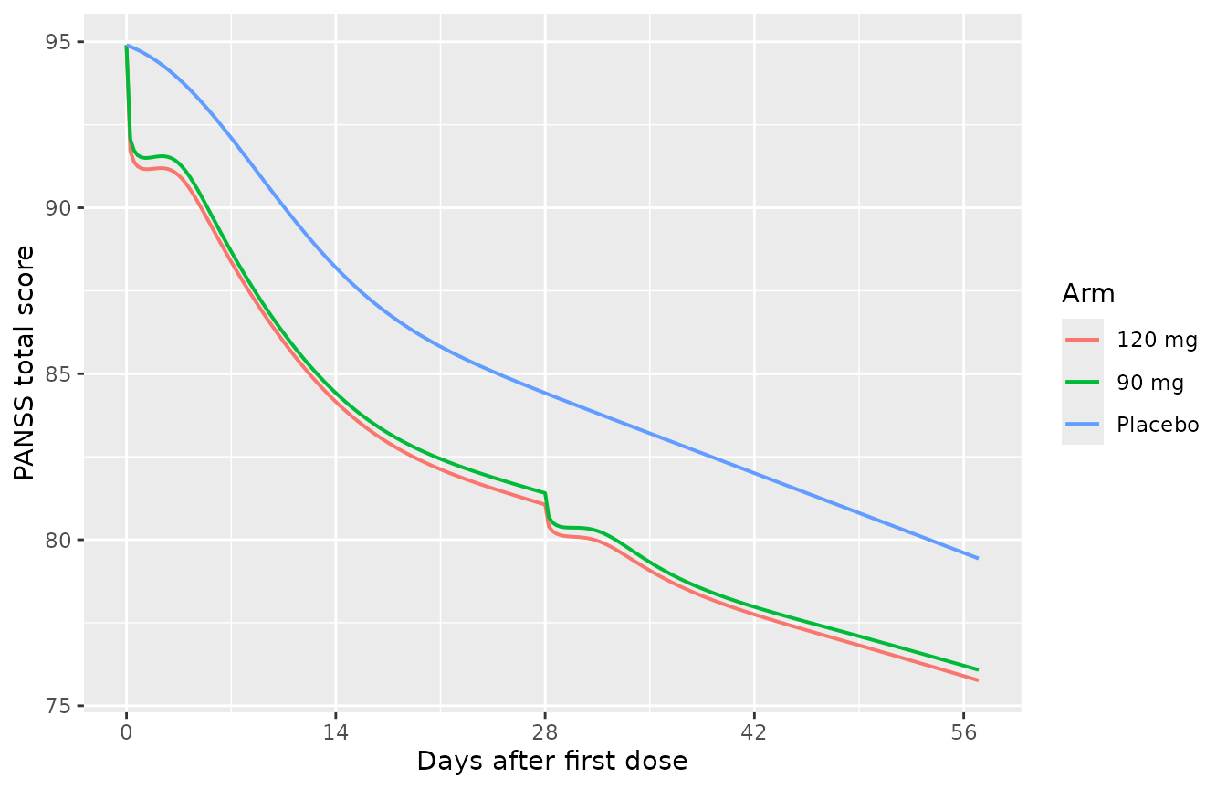
Replicates Figure 4 of Ivaturi 2017: typical-value PANSS total score over time after the first RBP-7000 dose, by treatment arm. Placebo trajectory is shown for reference by zeroing the AM (no drug) input via a third typical-value run with a sham 0 mg dose.
PKNCA validation
PKNCA is used to compute single-dose Cmax, Tmax, AUC, and half-life for the risperidone and 9-OH-risperidone outputs over the first 28-day dosing interval. The simulation uses the typical-value individual, so the NCA parameters represent the population typical exposure (not an inter-subject variability check; the sparse Phase 3 design and the typical-value simulation are not amenable to a full VPC reproducible here).
# Restrict to the first dosing interval (Day 0 to Day 28) and reshape to long.
# Per the canonical PKNCA recipe, do NOT filter `time > 0` or `Cc > 0` -- both
# drop the time-zero anchor row that AUC0-* requires; use only `!is.na(Cc)`.
sim_nca <- sim |>
  dplyr::filter(!is.na(Cc), time_day >= 0, time_day <= 28) |>
  dplyr::select(id, treatment, time_day, Cc, Cc_9oh) |>
  tidyr::pivot_longer(c(Cc, Cc_9oh), names_to = "analyte", values_to = "conc") |>
  dplyr::mutate(analyte = ifelse(analyte == "Cc", "risperidone", "9OH"))

# Guarantee a time = 0 row per (id, analyte, treatment); pre-dose is 0 ng/mL
# for an extravascular SC depot dose.
sim_nca <- dplyr::bind_rows(
  sim_nca,
  sim_nca |>
    dplyr::distinct(id, analyte, treatment) |>
    dplyr::mutate(time_day = 0, conc = 0)
) |>
  dplyr::distinct(id, analyte, treatment, time_day, .keep_all = TRUE) |>
  dplyr::arrange(id, analyte, treatment, time_day)

conc_obj <- PKNCA::PKNCAconc(
  sim_nca,
  conc ~ time_day | analyte + treatment / id,
  concu = "ng/mL",
  timeu = "day"
)

dose_df <- events |>
  dplyr::filter(evid == 1, time == 0) |>
  dplyr::mutate(time_day = time / 24, dose_amt = amt) |>
  dplyr::select(id, treatment, time_day, dose_amt)

dose_obj <- PKNCA::PKNCAdose(
  dose_df,
  dose_amt ~ time_day | treatment + id,
  doseu = "mg"
)

intervals <- data.frame(
  start      = 0,
  end        = 28,
  cmax       = TRUE,
  tmax       = TRUE,
  auclast    = TRUE,
  half.life  = TRUE
)

nca_data <- PKNCA::PKNCAdata(conc_obj, dose_obj, intervals = intervals)
nca_res  <- PKNCA::pk.nca(nca_data)
nca_df   <- as.data.frame(nca_res$result)
knitr::kable(
  nca_df |>
    dplyr::select(analyte, treatment, PPTESTCD, PPORRES) |>
    tidyr::pivot_wider(names_from = PPTESTCD, values_from = PPORRES),
  digits = 3,
  caption = "Single-dose NCA over the first 28-day dosing interval for the typical-value individual, by analyte and treatment arm."
)| analyte | treatment | auclast | cmax | tmax | tlast | lambda.z | r.squared | adj.r.squared | lambda.z.time.first | lambda.z.time.last | lambda.z.n.points | clast.pred | half.life | span.ratio |
|---|---|---|---|---|---|---|---|---|---|---|---|---|---|---|
| 9OH | 120 mg | 271.087 | 14.247 | 11.75 | 28 | 0.039 | 1 | 1 | 26.00 | 28 | 9 | 6.906 | 17.562 | 0.114 |
| 9OH | 90 mg | 203.315 | 10.685 | 11.75 | 28 | 0.039 | 1 | 1 | 26.00 | 28 | 9 | 5.180 | 17.562 | 0.114 |
| risperidone | 120 mg | 85.587 | 4.469 | 11.25 | 28 | 0.039 | 1 | 1 | 25.75 | 28 | 10 | 2.106 | 17.856 | 0.126 |
| risperidone | 90 mg | 64.190 | 3.352 | 11.25 | 28 | 0.039 | 1 | 1 | 25.75 | 28 | 10 | 1.580 | 17.856 | 0.126 |
The Ivaturi 2017 paper does not report a side-by-side NCA table for RBP-7000 (its Table 2 reports the popPK parameter estimates rather than NCA parameters). The mean concentration-time profiles in Figure 2 are the primary published validation target; the typical-value simulation above reproduces the dual-peak shape and the dose-proportional scaling between the 90 mg and 120 mg arms.
Assumptions and deviations
Dual-absorption dose encoding. Figure 1 of the source paper shows two parallel paths from the “Dose” box – a fast first-order route (ka1 directly to the risperidone central compartment) and a slow ATRIGEL-release route through a 5-compartment transit chain (ktr, with terminal ka2 into central). Table 2 / A2 report the rate constants but do NOT report an explicit bioavailability split between the two paths; the upstream Gomeni 2013 / Laffont 2014 / Laffont 2015 papers (where the structural model was originally developed) are not on disk. The package model encodes the simplest mass-conserving interpretation consistent with the Table 2 parameters: a single SC depot that simultaneously eliminates via ka1 (directly to central, fast-peak path) and via ktr (into transit1 of the chain, slow-peak path). The implicit fast-path fraction is then
ka1 / (ka1 + ktr)~ 18% and the slow-path fraction isktr / (ka1 + ktr)~ 82% at the typical-value estimates. This is one of several mathematically equivalent ways to express the dual-absorption pattern; if the upstream papers used a fitted F1 split with both depots receiving the full dose, the package model’s apparent V (129 L) absorbs the difference. The PANSS PK/PD output is unchanged because total active moiety is the integrating variable.CGI-S proportional-odds model not implemented. The paper also fits a CGI-S proportional-odds logistic-regression PD model (Section “Pharmacodynamic model for CGI-S”, Table 4) on the 4 consolidated CGI-S categories (3 = mildly ill, 4 = moderately ill, 5 = markedly ill, 6 = severely ill). The parameter estimates (intercepts alpha_4 = 8.5, alpha_5 = -6.5, alpha_6 = -6.4; time slope TSLP = -0.6 / week; concentration slope CSLP = -0.04 ng/mL^-1 on the logit) are documented in the source. rxode2’s additive-residual ODE pipeline does not natively express ordinal-logistic observation likelihoods, so the CGI-S sub-model is not implemented in the package model file. Users who need CGI-S predictions can compute the per-category probabilities externally from the simulated total active moiety trajectory using the Table 4 estimates:
logit(P(Y_ij >= m)) = alpha_m + TSLP * TIME_weeks + CSLP * AMfor m = 4, 5, 6.CYP2D6 reference category includes Inconclusive. Ivaturi 2017 Methods pools CYP2D6 Extensive Metabolizers and Inconclusive subjects as the covariate reference (both
CYP2D6_PM = 0andCYP2D6_IM = 0). Users simulating from this model who have an explicit “Inconclusive” stratum in their target population should code those subjects with both indicators 0 to match the reference. The pooled-reference approach reflects the small Inconclusive count in the Phase 3 cohort (5-7% across arms) and the paper’s covariate-modelling decision not to estimate a separate Inconclusive effect.Time-zero NCA anchor. The PKNCA inputs are augmented with a time = 0 Cc = 0 row per (id, analyte, treatment) so AUC0-t can anchor on the pre-dose baseline; this follows the canonical PKNCA recipe and is not a paper-derived addition.
No covariates retained on PK absorption / disposition or on PANSS PD beyond CYP2D6 on kr9. The paper screened age, body weight, BMI, waist-to-hip ratio, AST, ALT, creatinine clearance, sex, race, ethnicity, CYP2D6 phenotype, and four pharmacogenomic receptor genotypes (DRD2, 5-HT2A, 5-HT2C, MC4R); only the CYP2D6 phenotype effect on metabolite formation was retained. The screened-but-not-retained covariates are recorded under
covariatesDataExcludedrather thancovariateDatasocheckModelConventions()does not flag them as declared-but-unreferenced.