Adebrelimab (Chen 2024)
Source:vignettes/articles/Chen_2024_adebrelimab.Rmd
Chen_2024_adebrelimab.RmdModel and source
ui <- rxode2::rxode(readModelDb("Chen_2024_adebrelimab"))
#> ℹ parameter labels from comments will be replaced by 'label()'- Citation: Chen P, Zhang Y, Wang Y, Ma K, Shi W, Djebli N, Shen K. Population pharmacokinetics of adebrelimab - Support of alternative flat dose regimen in extensive-stage small-cell lung cancer. CPT Pharmacometrics Syst Pharmacol. 2024;13(7):1238-1251. doi:10.1002/psp4.13155
- Description: Two-compartment population PK model for adebrelimab (anti-PD-L1 IgG4) with empirical sigmoid time-varying clearance, fitted to 263 Chinese patients with extensive-stage small-cell lung cancer or advanced solid tumours from the phase I SHR-1316-I-101 and phase III CAPSTONE-1 (SHR-1316-III-301) studies (Chen 2024)
- Article: https://doi.org/10.1002/psp4.13155
- Supplement (Tables S1-S4, Code S1 NONMEM control stream, Code S2 R sampling code): https://doi.org/10.1002/psp4.13155 Supporting Information
Adebrelimab is an anti-PD-L1 IgG4 monoclonal antibody approved in China for extensive-stage small-cell lung cancer (ES-SCLC) in combination with carboplatin and etoposide. Chen 2024 built the first published population PK model for the drug and used it to support an alternative flat 1200 mg q3w regimen in place of the marketed 20 mg/kg q3w weight-based regimen.
The structural model is two-compartment with linear,
time-varying clearance described by an empirical
sigmoid maximal-change function of time since the first dose – the same
construct used for other immune checkpoint inhibitors (compare
modellib("Kuchimanchi_2024_dostarlimab"), which uses the
same functional form for dostarlimab).
Population
The analysis pooled 263 Chinese patients from two studies: 41 patients with advanced solid tumours from the phase I dose-escalation/expansion study (NCT03474289, SHR-1316-I-101, doses 3-20 mg/kg) and 222 patients with ES-SCLC from the pivotal phase III CAPSTONE-1 study (NCT03711305, SHR-1316-III-301, all at 20 mg/kg q3w with carboplatin and etoposide). Median age was 61 years (range 18-73), median baseline body weight 64.0 kg (range 38.1-97.0), and 25.1% were female. All patients were Asian (Chinese) and all had metastatic disease. Median albumin was 41.4 g/L and median neutrophil count 4.2 x 10^9/L; 27.0% of patients were positive for treatment-emergent anti-drug antibodies. Baseline demographics are Chen 2024 Table 1.
The same information is available programmatically from the model metadata:
str(ui$population, max.level = 1)
#> List of 18
#>  $ species               : chr "human"
#>  $ n_subjects            : int 263
#>  $ n_studies             : int 2
#>  $ age_range             : chr "18-73 years"
#>  $ age_median            : chr "61 years"
#>  $ weight_range          : chr "38.1-97.0 kg"
#>  $ weight_median         : chr "64.0 kg"
#>  $ sex_female_pct        : num 25.1
#>  $ race_ethnicity        : Named num 100
#>   ..- attr(*, "names")= chr "Asian_Chinese"
#>  $ disease_state         : chr "Extensive-stage small-cell lung cancer (222 patients from the phase III CAPSTONE-1 study, all receiving adebrel"| __truncated__
#>  $ dose_range            : chr "3 mg/kg q3w (n = 3), 10 mg/kg q2w (n = 12), 10 mg/kg q3w (n = 13), and 20 mg/kg q3w (n = 235) as intravenous infusions"
#>  $ regions               : chr "China"
#>  $ ada_positive_pct      : num 27
#>  $ albumin_median        : chr "41.4 g/L (range 26.6-53.2)"
#>  $ neutrophil_median     : chr "4.2 x 10^9/L (range 1.7-11.4)"
#>  $ hepatic_impairment_pct: Named num [1:4] 84 15.2 0.8 0
#>   ..- attr(*, "names")= chr [1:4] "none" "mild" "moderate" "severe"
#>  $ renal_impairment_pct  : Named num [1:4] 51 39.5 9.5 0
#>   ..- attr(*, "names")= chr [1:4] "none" "mild" "moderate" "severe"
#>  $ notes                 : chr "Baseline demographics from Chen 2024 Table 1 (total population column, N = 263). Studies: NCT03474289 (SHR-1316"| __truncated__
Source trace
Every ini() entry carries an in-file comment naming its
source. The final model’s point estimates were taken from the
Code S1 NONMEM control stream in the Supporting
Information, which reports more significant figures than the rounded
Chen 2024 Table 2 values; both are listed below and they agree.
| Equation / parameter | Value | Source location |
|---|---|---|
d/dt(central), d/dt(peripheral1)
|
n/a | Two-compartment linear disposition; Code S1
$SUBROUTINE ADVAN3 TRANS4
|
CL(t) = TVCL * exp(Imax * t^HILL / (TC50^HILL + t^HILL)) |
n/a | Chen 2024 Equation 1; Code S1 $PK sigmoid time-varying
CL line |
Par = Par_ref * (Cov / Cov_median)^theta |
n/a | Chen 2024 Equation 3 (continuous covariates) |
Par = Par_ref * (1 + theta) |
n/a | Chen 2024 Equation 4 (categorical covariates) |
lcl (CL) |
0.237784 L/day | Code S1 $THETA(1); Table 2 = 0.238 |
lvc (V1) |
3.22559 L | Code S1 $THETA(2); Table 2 = 3.23 |
lq (Q) |
0.703417 L/day | Code S1 $THETA(3); Table 2 = 0.703 |
lvp (V2) |
1.69298 L | Code S1 $THETA(4); Table 2 = 1.69 |
cl_time_max (Imax) |
-0.34925 | Code S1 $THETA(5); Table 2 = -0.349 |
lcl_t50 (TC50) |
74.4482 day | Code S1 $THETA(6); Table 2 = 74.4 |
lcl_time_hill (HILL) |
1.96911 | Code S1 $THETA(7); Table 2 = 1.97 |
e_ada_pos_cl |
0.185112 | Code S1 $THETA(8); Table 2 = 0.185 |
e_alb_cl |
-0.861333 | Code S1 $THETA(9); Table 2 = -0.861 |
e_wt_cl |
0.70974 | Code S1 $THETA(10); Table 2 = 0.710 |
e_neut_cl |
0.158825 | Code S1 $THETA(11); Table 2 = 0.159 |
e_tum_sld_cl |
0.102909 | Code S1 $THETA(12); Table 2 = 0.103 |
e_wt_vc |
0.576703 | Code S1 $THETA(13); Table 2 = 0.577 |
e_wt_vp |
1.79986 | Code S1 $THETA(14); Table 2 = 1.8 |
| Covariate normalisers 64 kg / 41.4 g/L / 4.15 x 10^9 per L / 90 mm | n/a | Code S1 $PK covariate block (hard-coded divisors) |
| IIV block on CL, V1, V2 | 0.0415871; 0.0104212, 0.0296031; 0.0370675, 0.0308242, 0.128194 | Code S1 $OMEGA BLOCK(3); Table 2 IIV / Cov rows |
| IIV on Imax (additive eta) | 0.0533643 | Code S1 second $OMEGA; Table 2 = 0.0534 |
propSd |
sqrt(0.0223852) = 0.149617 | Code S1 $SIGMA(1); Table 2 sigma^2_Prop = 0.0224 |
addSd |
sqrt(32.6463) = 5.71370 ug/mL | Code S1 $SIGMA(2); Table 2 sigma^2_add = 32.6 |
| Covariate 5th / 95th percentiles used below | see cohort chunk | Chen 2024 Figure 1 left-hand labels |
| Published exposure comparisons | see tables below | Chen 2024 Tables S2, S3, S4 |
Structural identity checks
Three quantities in the paper are exact algebraic consequences of the parameter values, so they validate the transcription independently of any simulated cohort. These are deterministic and are asserted tightly.
th <- setNames(ui$theta, names(ui$theta))
cl0 <- exp(th[["lcl"]]); vc <- exp(th[["lvc"]])
vp  <- exp(th[["lvp"]]); q  <- exp(th[["lq"]])
imax <- th[["cl_time_max"]]

# 1. Volume of distribution at steady state = V1 + V2.
vss <- vc + vp

# 2. Asymptotic fractional CL remaining at t >> TC50 is exp(Imax); the paper
#    reports geometric-mean CL falling from 0.25 to 0.177 L/day.
cl_decay_model <- exp(imax)
cl_decay_paper <- 0.177 / 0.25

# 3. Terminal (beta) half-life of the two-compartment system evaluated at the
#    reported steady-state clearance.
kel <- (0.25 * cl_decay_model) / vc; k12 <- q / vc; k21 <- q / vp
s <- kel + k12 + k21
beta <- 0.5 * (s - sqrt(s^2 - 4 * kel * k21))
thalf <- log(2) / beta

identities <- tibble::tibble(
  Quantity  = c("Vss = V1 + V2 (L)", "CL(ss) / CL(baseline)",
                "Terminal half-life at steady state (day)"),
  Model     = c(vss, cl_decay_model, thalf),
  Published = c(4.91, cl_decay_paper, 19.9),
  Source    = c("Chen 2024 Results", "Chen 2024 Results (0.177 / 0.25 L/day)",
                "Chen 2024 Results")
) |>
  mutate(`Difference (%)` = 100 * (Model / Published - 1))

knitr::kable(identities, digits = c(0, 4, 4, 0, 2),
caption = "Algebraic identities implied by the parameter values.")| Quantity | Model | Published | Source | Difference (%) |
|---|---|---|---|---|
| Vss = V1 + V2 (L) | 4.9186 | 4.910 | Chen 2024 Results | 0.17 |
| CL(ss) / CL(baseline) | 0.7052 | 0.708 | Chen 2024 Results (0.177 / 0.25 L/day) | -0.39 |
| Terminal half-life at steady state (day) | 19.9451 | 19.900 | Chen 2024 Results | 0.23 |
Replicating Figure 1a: covariate forest plot
Chen 2024 Figure 1 reports the fold change in steady-state exposure for each covariate at its 5th and 95th percentiles relative to a reference patient at the covariate medians. The forest plot was generated from typical-value simulations, so it can be reproduced exactly with the random effects zeroed – every subject-level and residual source of variability cancels in the ratio. This is the single strongest check on the covariate block: it exercises every coefficient, every median normaliser, every functional form and every sign.
Body weight is evaluated under the marketed 20 mg/kg regimen, so the dose scales with weight in that row.
mod_typ <- rxode2::zeroRe(ui)

ref <- list(WT = 64, ALB = 41.4, NEUT = 4150, TUM_SLD = 90, ADA_POS = 0)

# Chen 2024 Figure 1 left-hand labels give the 5th / 95th percentiles. NEUT is
# labelled in 10^9/L and is carried here in the canonical cells/mm^3
# (x 1000); SLD is labelled in mm.
conditions <- tibble::tribble(
  ~label,             ~covariate, ~value,  ~auc_ratio, ~cmax_ratio, ~ctrough_ratio,
  "ADA positive",     "ADA_POS",   1,       0.84,       0.92,        0.78,
  "ALB 48.29 g/L",    "ALB",       48.29,   1.14,       1.08,        1.20,
  "ALB 33.06 g/L",    "ALB",       33.06,   0.82,       0.91,        0.75,
  "BW 84.27 kg",      "WT",        84.27,   1.08,       1.12,        1.10,
  "BW 47.1 kg",       "WT",        47.1,    0.91,       0.89,        0.90,
  "NEUT 7.781e9/L",   "NEUT",      7781,    0.91,       0.95,        0.87,
  "NEUT 2.381e9/L",   "NEUT",      2381,    1.09,       1.05,        1.13,
  "SLD 176.75 mm",    "TUM_SLD",   176.75,  0.93,       0.96,        0.91,
  "SLD 28.03 mm",     "TUM_SLD",   28.03,   1.13,       1.07,        1.18
)

# Steady state is cycle 20, matching the paper ("at 20th administration
# cycles"). Observations are placed on the ODE state `central`; rxode2 returns
# the algebraic observable Cc as a column at those rows.
ss_events <- function(covs, id) {
  ev <- dplyr::bind_rows(
    tibble::tibble(time = seq(0, by = 21, length.out = 20),
                   amt = 20 * covs$WT, evid = 1L, dur = 1 / 24),
    tibble::tibble(time = seq(19 * 21, 20 * 21, by = 0.25),
                   amt = NA_real_, evid = 0L, dur = NA_real_)
  ) |>
    dplyr::mutate(id = id, cmt = "central", WT = covs$WT, ALB = covs$ALB,
                  NEUT = covs$NEUT, TUM_SLD = covs$TUM_SLD,
                  ADA_POS = covs$ADA_POS) |>
    dplyr::arrange(time, dplyr::desc(evid))
  ev
}

all_covs <- c(
  list(ref),
  lapply(seq_len(nrow(conditions)), function(i) {
    x <- ref
    x[[conditions$covariate[i]]] <- conditions$value[i]
    x
  })
)

forest_events <- dplyr::bind_rows(
  lapply(seq_along(all_covs), function(i) ss_events(all_covs[[i]], id = i))
)
stopifnot(!anyDuplicated(unique(forest_events[, c("id", "time", "evid")])))

forest_sim <- rxode2::rxSolve(mod_typ, forest_events,
                              returnType = "data.frame")
#> ℹ omega/sigma items treated as zero: 'etalcl', 'etalvc', 'etalvp', 'etacl_time_max'
#> Warning: multi-subject simulation without without 'omega'

metrics <- forest_sim |>
  dplyr::arrange(id, time) |>
  dplyr::group_by(id) |>
  dplyr::summarise(
    auc     = sum(diff(time) * (head(Cc, -1) + tail(Cc, -1)) / 2),
    cmax    = max(Cc),
    ctrough = dplyr::last(Cc),
    .groups = "drop"
  )

reference_row <- metrics[metrics$id == 1, ]
forest <- conditions |>
  dplyr::mutate(
    `AUCtau,ss (model)`   = metrics$auc[-1]     / reference_row$auc,
    `Cmax,ss (model)`     = metrics$cmax[-1]    / reference_row$cmax,
    `Ctrough,ss (model)`  = metrics$ctrough[-1] / reference_row$ctrough
  )

forest |>
  dplyr::select(label,
                `AUCtau,ss (model)`, auc_ratio,
                `Cmax,ss (model)`, cmax_ratio,
                `Ctrough,ss (model)`, ctrough_ratio) |>
  dplyr::rename(
    "Condition"              = label,
    "AUCtau,ss (published)"  = auc_ratio,
    "Cmax,ss (published)"    = cmax_ratio,
    "Ctrough,ss (published)" = ctrough_ratio
  ) |>
  knitr::kable(
    digits = 3,
    caption = paste("Replicates Figure 1 of Chen 2024: fold change in",
                    "steady-state exposure relative to the median-covariate",
                    "reference patient.")
)| Condition | AUCtau,ss (model) | AUCtau,ss (published) | Cmax,ss (model) | Cmax,ss (published) | Ctrough,ss (model) | Ctrough,ss (published) |
|---|---|---|---|---|---|---|
| ADA positive | 0.843 | 0.84 | 0.913 | 0.92 | 0.782 | 0.78 |
| ALB 48.29 g/L | 1.142 | 1.14 | 1.080 | 1.08 | 1.201 | 1.20 |
| ALB 33.06 g/L | 0.823 | 0.82 | 0.902 | 0.91 | 0.754 | 0.75 |
| BW 84.27 kg | 1.083 | 1.08 | 1.119 | 1.12 | 1.100 | 1.10 |
| BW 47.1 kg | 0.915 | 0.91 | 0.882 | 0.89 | 0.897 | 0.90 |
| NEUT 7.781e9/L | 0.905 | 0.91 | 0.947 | 0.95 | 0.867 | 0.87 |
| NEUT 2.381e9/L | 1.092 | 1.09 | 1.052 | 1.05 | 1.131 | 1.13 |
| SLD 176.75 mm | 0.933 | 0.93 | 0.963 | 0.96 | 0.906 | 0.91 |
| SLD 28.03 mm | 1.128 | 1.13 | 1.072 | 1.07 | 1.181 | 1.18 |
forest |>
  dplyr::select(label, model = `AUCtau,ss (model)`, published = auc_ratio) |>
  tidyr::pivot_longer(c(model, published), names_to = "source",
                      values_to = "ratio") |>
  ggplot(aes(x = ratio, y = label, colour = source, shape = source)) +
  annotate("rect", xmin = 0.8, xmax = 1.25, ymin = -Inf, ymax = Inf,
           alpha = 0.15) +
  geom_vline(xintercept = 1, linetype = "dashed") +
  geom_point(size = 2.5, position = position_dodge(width = 0.4)) +
  labs(x = "Fold change of AUCtau,ss relative to reference", y = NULL,
       title = "Figure 1a - covariate effects on steady-state AUC",
       caption = paste("Replicates Figure 1a of Chen 2024. Shaded band is the",
                       "80-125% no-effect range.")) +
  theme(legend.position = "bottom")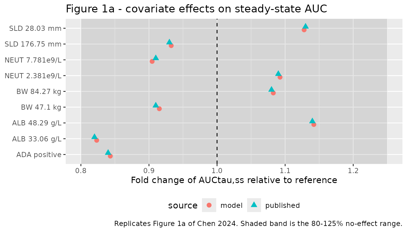
pct <- 100 * c(forest$`AUCtau,ss (model)` / forest$auc_ratio,
               forest$`Cmax,ss (model)` / forest$cmax_ratio,
               forest$`Ctrough,ss (model)` / forest$ctrough_ratio) - 100

# Deterministic typical-value ratios: no cohort is drawn and no RNG is used, so
# the only error source is the paper rounding its ratios to two decimals (up to
# ~0.6% on a ratio near 0.8). A mis-transcribed exponent, normaliser or sign
# moves a row by many percent, so this gate stays tight.
stopifnot(max(abs(pct)) < 2)
Replicating Figure S5: time-varying clearance
cl_profile <- tibble::tibble(time = seq(0, 420, by = 1)) |>
  dplyr::mutate(
    hill = exp(th[["lcl_time_hill"]]),
    t50  = exp(th[["lcl_t50"]]),
    `CL(t) / CL(0)` = exp(imax * time^hill / (t50^hill + time^hill))
  )

ggplot(cl_profile, aes(time, `CL(t) / CL(0)`)) +
  geom_line(linewidth = 0.8) +
  geom_hline(yintercept = exp(imax), linetype = "dashed") +
  labs(x = "Time since first dose (day)", y = "CL(t) / CL(0)",
       title = "Figure S5 - typical time course of clearance",
       caption = paste0("Replicates Figure S5 of Chen 2024. Dashed line is",
                        " the asymptote exp(Imax) = ",
                        sprintf("%.3f", exp(imax)), "."))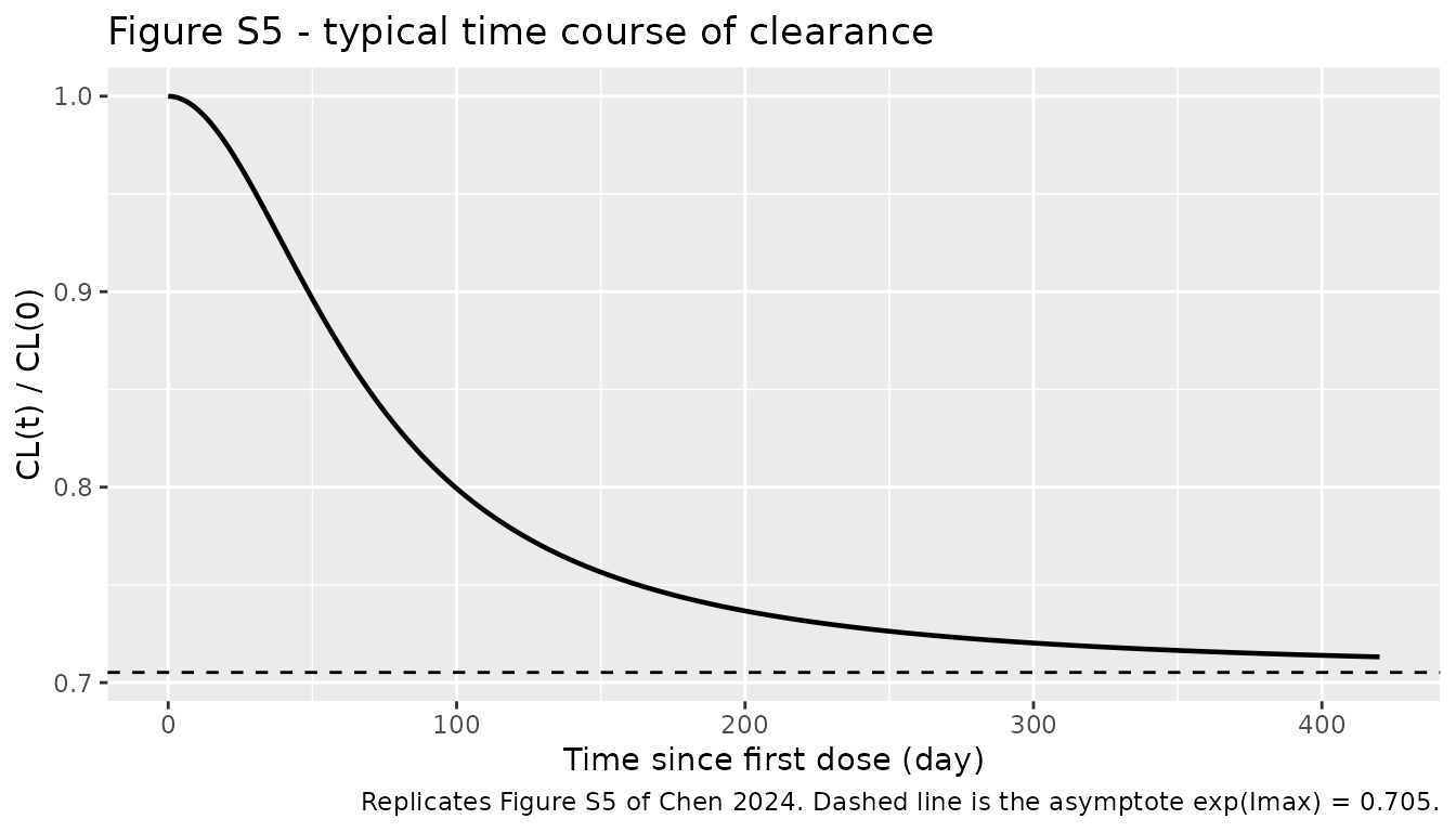
Virtual cohort
Individual patient data are not public. The cohort below reproduces the marginal covariate distributions of Chen 2024 Table 1 and the 5th / 95th percentiles printed in Figure 1, truncated to the reported ranges.
Both dosing regimens are applied to the same virtual
patients, matching the paper’s simulation design (Code S2 resamples one
covariate/parameter pool and applies both regimens to it). To pair the
arms exactly, the random effects are drawn once in base R and supplied
to rxSolve() as data columns with omega = NA;
drawing them inside rxSolve() would give each arm an
independent draw and silently break the paired comparison.
set.seed(20240715)
n_sub <- 200  # per arm; the two arms share these subjects

rtrunc_lnorm <- function(n, median, sdlog, lower, upper) {
  x <- stats::rlnorm(n, log(median), sdlog)
  pmin(pmax(x, lower), upper)
}

subj <- tibble::tibble(
  subject = seq_len(n_sub),
  # Table 1: median 64.0 kg, range 38.1-97.0; Figure 1: 5th 47.1, 95th 84.27.
  WT      = rtrunc_lnorm(n_sub, 64, 0.177, 38.1, 97.0),
  # Table 1: median 41.4 g/L, range 26.6-53.2; Figure 1: 5th 33.06, 95th 48.29.
  ALB     = pmin(pmax(stats::rnorm(n_sub, 41.4, 4.6), 26.6), 53.2),
  # Table 1 median 4.2e9/L, range 1.7-11.4e9/L; Figure 1 5th 2.381, 95th 7.781.
  # Carried in the canonical cells/mm^3 (= 10^9/L x 1000).
  NEUT    = rtrunc_lnorm(n_sub, 4150, 0.36, 1700, 11400),
  # Not tabulated by Chen 2024; median 90 mm from the Code S1 normaliser,
  # spread from the Figure 1 percentiles (28.03 / 176.75 mm).
  TUM_SLD = rtrunc_lnorm(n_sub, 90, 0.50, 20, 260),
  # Table 1: 71 of 263 evaluable patients (27.0%) ADA-positive.
  ADA_POS = stats::rbinom(n_sub, 1, 0.270)
)

# Random effects drawn ONCE, shared by both regimens.
omega_block <- matrix(c(0.0415871, 0.0104212, 0.0370675,
                        0.0104212, 0.0296031, 0.0308242,
                        0.0370675, 0.0308242, 0.128194), nrow = 3)
eta_block <- mvtnorm::rmvnorm(n_sub, mean = rep(0, 3), sigma = omega_block)
subj <- subj |>
  dplyr::mutate(
    etalcl         = eta_block[, 1],
    etalvc         = eta_block[, 2],
    etalvp         = eta_block[, 3],
    # Chen 2024 gives Imax a NORMAL distribution with an ADDITIVE eta.
    etacl_time_max = stats::rnorm(n_sub, 0, sqrt(0.0533643))
  )

summary_tab <- subj |>
  dplyr::summarise(
    `WT (kg)`          = sprintf("%.1f (%.1f-%.1f)", median(WT), min(WT), max(WT)),
    `ALB (g/L)`        = sprintf("%.1f (%.1f-%.1f)", median(ALB), min(ALB), max(ALB)),
    `NEUT (10^9/L)`    = sprintf("%.2f (%.2f-%.2f)", median(NEUT) / 1000,
                                 min(NEUT) / 1000, max(NEUT) / 1000),
    `TUM_SLD (mm)`     = sprintf("%.0f (%.0f-%.0f)", median(TUM_SLD),
                                 min(TUM_SLD), max(TUM_SLD)),
    `ADA positive (%)` = sprintf("%.1f", 100 * mean(ADA_POS))
  ) |>
  tidyr::pivot_longer(everything(), names_to = "Covariate",
                      values_to = "Simulated: median (range)")

summary_tab |>
  dplyr::mutate(
    `Chen 2024 Table 1` = c("64.0 (38.1-97.0)", "41.4 (26.6-53.2)",
                            "4.20 (1.70-11.40)", "not tabulated", "27.0")
  ) |>
knitr::kable(caption = "Virtual cohort versus the published demographics.")| Covariate | Simulated: median (range) | Chen 2024 Table 1 |
|---|---|---|
| WT (kg) | 62.9 (38.1-97.0) | 64.0 (38.1-97.0) |
| ALB (g/L) | 42.0 (29.6-53.2) | 41.4 (26.6-53.2) |
| NEUT (10^9/L) | 4.20 (1.72-9.20) | 4.20 (1.70-11.40) |
| TUM_SLD (mm) | 87 (30-260) | not tabulated |
| ADA positive (%) | 27.0 | 27.0 |
Simulation: flat versus weight-based dosing
# 20 cycles q3w. Observations cover the first dosing interval (for the
# published AUC0-21day / Cmax / Ctrough) and cycle 20 (steady state, matching
# the paper's "at 20th administration cycles"). The trough sample sits at
# 20.99 day so it precedes the next dose.
cycle1_times <- c(0, 1 / 24, 0.125, 0.25, 0.5, 1, 2, 3, 5, 7, 10, 14, 17, 20.99)
ss_times     <- seq(19 * 21, 19 * 21 + 20.99, by = 0.5)

make_arm <- function(regimen, id_offset) {
  dose_amt <- if (regimen == "1200 mg q3w") rep(1200, n_sub) else 20 * subj$WT
  doses <- subj |>
    dplyr::mutate(id = subject + id_offset, amt = dose_amt) |>
    tidyr::crossing(time = seq(0, by = 21, length.out = 20)) |>
    dplyr::mutate(evid = 1L, dur = 1 / 24)
  obs <- subj |>
    dplyr::mutate(id = subject + id_offset, amt = NA_real_) |>
    tidyr::crossing(time = c(cycle1_times, ss_times)) |>
    dplyr::mutate(evid = 0L, dur = NA_real_)
  dplyr::bind_rows(doses, obs) |>
    dplyr::mutate(cmt = "central", regimen = regimen) |>
    dplyr::arrange(id, time, dplyr::desc(evid))
}

events <- dplyr::bind_rows(
  make_arm("20 mg/kg q3w", id_offset = 0L),
  make_arm("1200 mg q3w",  id_offset = n_sub)
)
stopifnot(!anyDuplicated(unique(events[, c("id", "time", "evid")])))
# omega = NA / sigma = NA: the etas ride in as data columns (see the cohort
# chunk), so both arms see identical subject-level random effects.
sim <- rxode2::rxSolve(
  ui, events, omega = NA, sigma = NA,
  keep = c("regimen", "WT", "ALB", "NEUT", "TUM_SLD", "ADA_POS"),
  returnType = "data.frame"
)
stopifnot(all(sim$Cc >= 0), !anyNA(sim$Cc))
geomean <- function(x) exp(mean(log(x)))
geocv   <- function(x) 100 * sqrt(exp(stats::var(log(x))) - 1)

cycle1 <- sim |>
  dplyr::filter(time <= 20.99) |>
  dplyr::arrange(id, time)
ss <- sim |>
  dplyr::filter(time >= 19 * 21) |>
  dplyr::arrange(id, time)

trapz <- function(t, y) sum(diff(t) * (head(y, -1) + tail(y, -1)) / 2)

exposure <- dplyr::bind_rows(
  cycle1 |>
    dplyr::group_by(id, regimen, WT) |>
    dplyr::summarise(AUC = trapz(time, Cc), Cmax = max(Cc),
                     Ctrough = dplyr::last(Cc), .groups = "drop") |>
    dplyr::mutate(interval = "First dose"),
  ss |>
    dplyr::group_by(id, regimen, WT) |>
    dplyr::summarise(AUC = trapz(time, Cc), Cmax = max(Cc),
                     Ctrough = dplyr::last(Cc), .groups = "drop") |>
    dplyr::mutate(interval = "Steady state (cycle 20)")
) |>
  dplyr::mutate(
    wt_quartile = cut(WT, breaks = stats::quantile(subj$WT, c(0, .25, .5, .75, 1)),
                      include.lowest = TRUE)
  )
exposure |>
  ggplot(aes(x = regimen, y = AUC, fill = regimen)) +
  geom_boxplot(alpha = 0.7, outlier.size = 0.6) +
  facet_grid(interval ~ wt_quartile, scales = "free_y") +
  scale_y_log10() +
  labs(x = NULL, y = "AUC (ug*day/mL)",
       title = "Figure 5 - simulated exposure by body-weight quartile",
       caption = paste("Replicates Figure 5b,d of Chen 2024: AUC0-21day and",
                       "AUCtau,ss by weight quartile for the flat and",
                       "weight-based regimens.")) +
  theme(legend.position = "bottom", axis.text.x = element_blank(),
        axis.ticks.x = element_blank())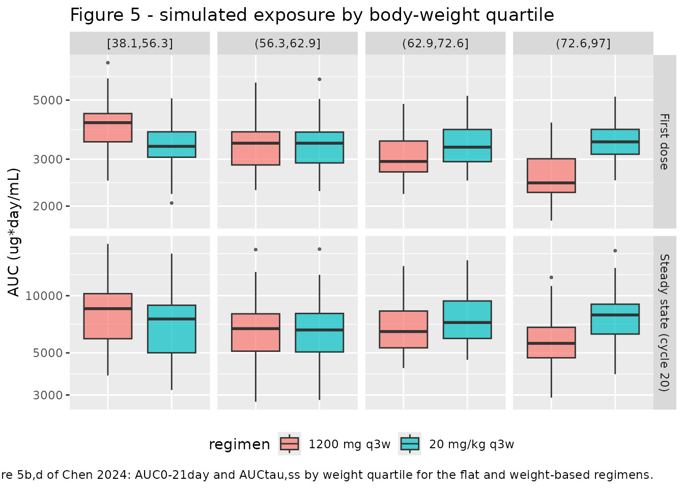
PKNCA validation
NCA is run on the first dosing interval, which is the window the
paper’s AUC0-21day refers to (Chen 2024 chose first-dose
exposure precisely because the time-varying clearance makes steady-state
metrics a biased predictor in the exposure-efficacy analysis).
sim_nca <- sim |>
  dplyr::filter(!is.na(Cc)) |>
  dplyr::filter(time <= 20.99) |>
  dplyr::select(id, time, Cc, regimen)

# Guarantee a time = 0 row per (id, regimen). For an IV infusion the pre-dose
# concentration is 0.
sim_nca <- dplyr::bind_rows(
  sim_nca,
  sim_nca |> dplyr::distinct(id, regimen) |>
    dplyr::mutate(time = 0, Cc = 0)
) |>
  dplyr::distinct(id, regimen, time, .keep_all = TRUE) |>
  dplyr::arrange(id, regimen, time)

conc_obj <- PKNCA::PKNCAconc(sim_nca, Cc ~ time | regimen + id)

dose_df <- events |>
  dplyr::filter(evid == 1, time == 0) |>
  dplyr::select(id, time, amt, regimen)
dose_obj <- PKNCA::PKNCAdose(dose_df, amt ~ time | regimen + id)

intervals <- data.frame(
  start = 0, end = 20.99,
  cmax = TRUE, tmax = TRUE, auclast = TRUE, clast.obs = TRUE
)

nca_res <- PKNCA::pk.nca(PKNCA::PKNCAdata(conc_obj, dose_obj,
                                          intervals = intervals))

nca_wide <- as.data.frame(nca_res) |>
  dplyr::select(regimen, id, PPTESTCD, PPORRES) |>
  tidyr::pivot_wider(names_from = PPTESTCD, values_from = PPORRES)
stopifnot(nrow(nca_wide) == 2 * n_sub)

nca_summary <- nca_wide |>
  dplyr::group_by(regimen) |>
  dplyr::summarise(
    `AUC0-21day geomean (geoCV%)` = sprintf("%.0f (%.1f)", geomean(auclast),
                                            geocv(auclast)),
    `Cmax geomean (geoCV%)`       = sprintf("%.0f (%.1f)", geomean(cmax),
                                            geocv(cmax)),
    `Ctrough geomean (geoCV%)`    = sprintf("%.1f (%.1f)", geomean(clast.obs),
                                            geocv(clast.obs)),
    `Tmax median (day)`           = sprintf("%.3f", median(tmax)),
    .groups = "drop"
  ) |>
  dplyr::rename("Regimen" = regimen)

knitr::kable(nca_summary,
caption = "PKNCA results over the first dosing interval.")| Regimen | AUC0-21day geomean (geoCV%) | Cmax geomean (geoCV%) | Ctrough geomean (geoCV%) | Tmax median (day) |
|---|---|---|---|---|
| 1200 mg q3w | 3185 (25.8) | 375 (20.9) | 80.1 (33.3) | 0.042 |
| 20 mg/kg q3w | 3383 (19.7) | 398 (19.9) | 85.0 (28.1) | 0.042 |
Comparison against the published simulations
Chen 2024 Tables S2-S4 report the geometric mean (geoCV%) of each exposure metric for both regimens over their 1000-patient virtual population. Those are the directly comparable numbers, because both they and the table below are model simulations over a resampled covariate distribution.
published <- tibble::tribble(
  ~Metric,                 ~Interval,                 ~regimen,        ~pub_geomean, ~pub_geocv, ~Source,
  "AUC (ug*day/mL)",       "First dose",              "20 mg/kg q3w",  3280,         20.0,       "Table S2",
  "AUC (ug*day/mL)",       "First dose",              "1200 mg q3w",   3110,         23.2,       "Table S2",
  "AUC (ug*day/mL)",       "Steady state (cycle 20)", "20 mg/kg q3w",  7080,         37.1,       "Table S2",
  "AUC (ug*day/mL)",       "Steady state (cycle 20)", "1200 mg q3w",   6710,         37.7,       "Table S2",
  "Cmax (ug/mL)",          "First dose",              "20 mg/kg q3w",  387,          24.8,       "Table S3",
  "Cmax (ug/mL)",          "First dose",              "1200 mg q3w",   367,          25.2,       "Table S3",
  "Cmax (ug/mL)",          "Steady state (cycle 20)", "20 mg/kg q3w",  618,          28.5,       "Table S3",
  "Cmax (ug/mL)",          "Steady state (cycle 20)", "1200 mg q3w",   586,          28.8,       "Table S3",
  "Ctrough (ug/mL)",       "First dose",              "20 mg/kg q3w",  80.2,         36.8,       "Table S4",
  "Ctrough (ug/mL)",       "First dose",              "1200 mg q3w",   76.0,         38.4,       "Table S4",
  "Ctrough (ug/mL)",       "Steady state (cycle 20)", "20 mg/kg q3w",  212,          57.7,       "Table S4",
  "Ctrough (ug/mL)",       "Steady state (cycle 20)", "1200 mg q3w",   201,          57.2,       "Table S4"
)

simulated <- exposure |>
  tidyr::pivot_longer(c(AUC, Cmax, Ctrough), names_to = "metric",
                      values_to = "value") |>
  dplyr::mutate(Metric = dplyr::recode(metric,
    AUC = "AUC (ug*day/mL)", Cmax = "Cmax (ug/mL)",
    Ctrough = "Ctrough (ug/mL)")) |>
  dplyr::group_by(Metric, Interval = interval, regimen) |>
  dplyr::summarise(sim_geomean = geomean(value), sim_geocv = geocv(value),
                   .groups = "drop")

cmp <- published |>
  dplyr::inner_join(simulated, by = c("Metric", "Interval", "regimen")) |>
  dplyr::mutate(`Difference (%)` = 100 * (sim_geomean / pub_geomean - 1))
stopifnot(nrow(cmp) == nrow(published))

cmp |>
  dplyr::select(Metric, Interval, regimen, sim_geomean, pub_geomean,
                sim_geocv, pub_geocv, `Difference (%)`, Source) |>
  dplyr::rename(
    "Regimen"            = regimen,
    "Model geomean"      = sim_geomean,
    "Published geomean"  = pub_geomean,
    "Model geoCV%"       = sim_geocv,
    "Published geoCV%"   = pub_geocv
  ) |>
  knitr::kable(digits = c(0, 0, 0, 1, 1, 1, 1, 1, 0),
               caption = paste("Simulated versus published exposure metrics",
"(Chen 2024 Tables S2-S4)."))| Metric | Interval | Regimen | Model geomean | Published geomean | Model geoCV% | Published geoCV% | Difference (%) | Source |
|---|---|---|---|---|---|---|---|---|
| AUC (ug*day/mL) | First dose | 20 mg/kg q3w | 3390.3 | 3280.0 | 19.7 | 20.0 | 3.4 | Table S2 |
| AUC (ug*day/mL) | First dose | 1200 mg q3w | 3192.4 | 3110.0 | 25.8 | 23.2 | 2.6 | Table S2 |
| AUC (ug*day/mL) | Steady state (cycle 20) | 20 mg/kg q3w | 7163.7 | 7080.0 | 35.3 | 37.1 | 1.2 | Table S2 |
| AUC (ug*day/mL) | Steady state (cycle 20) | 1200 mg q3w | 6745.6 | 6710.0 | 38.0 | 37.7 | 0.5 | Table S2 |
| Cmax (ug/mL) | First dose | 20 mg/kg q3w | 398.1 | 387.0 | 19.9 | 24.8 | 2.9 | Table S3 |
| Cmax (ug/mL) | First dose | 1200 mg q3w | 374.9 | 367.0 | 20.9 | 25.2 | 2.1 | Table S3 |
| Cmax (ug/mL) | Steady state (cycle 20) | 20 mg/kg q3w | 590.6 | 618.0 | 23.8 | 28.5 | -4.4 | Table S3 |
| Cmax (ug/mL) | Steady state (cycle 20) | 1200 mg q3w | 556.1 | 586.0 | 25.6 | 28.8 | -5.1 | Table S3 |
| Ctrough (ug/mL) | First dose | 20 mg/kg q3w | 85.0 | 80.2 | 28.1 | 36.8 | 6.0 | Table S4 |
| Ctrough (ug/mL) | First dose | 1200 mg q3w | 80.1 | 76.0 | 33.3 | 38.4 | 5.3 | Table S4 |
| Ctrough (ug/mL) | Steady state (cycle 20) | 20 mg/kg q3w | 229.7 | 212.0 | 50.1 | 57.7 | 8.3 | Table S4 |
| Ctrough (ug/mL) | Steady state (cycle 20) | 1200 mg q3w | 216.2 | 201.0 | 51.7 | 57.2 | 7.6 | Table S4 |
The headline claim of the paper is that the flat and weight-based regimens give similar exposure. That claim is a ratio between the two arms, so it is far more robust than either arm’s absolute level – the covariate distribution we had to approximate cancels almost entirely.
ratio_tab <- cmp |>
  dplyr::select(Metric, Interval, regimen, sim_geomean, pub_geomean) |>
  tidyr::pivot_wider(names_from = regimen,
                     values_from = c(sim_geomean, pub_geomean)) |>
  dplyr::mutate(
    `Model flat / weight-based`     = `sim_geomean_1200 mg q3w` /
                                      `sim_geomean_20 mg/kg q3w`,
    `Published flat / weight-based` = `pub_geomean_1200 mg q3w` /
                                      `pub_geomean_20 mg/kg q3w`
  )

ratio_tab |>
  dplyr::select(Metric, Interval, `Model flat / weight-based`,
                `Published flat / weight-based`) |>
  knitr::kable(digits = 3,
               caption = paste("Flat versus weight-based exposure ratio.",
                               "The FDA criterion cited by Chen 2024 is that",
"the geometric means agree within 20%."))| Metric | Interval | Model flat / weight-based | Published flat / weight-based |
|---|---|---|---|
| AUC (ug*day/mL) | First dose | 0.942 | 0.948 |
| AUC (ug*day/mL) | Steady state (cycle 20) | 0.942 | 0.948 |
| Cmax (ug/mL) | First dose | 0.942 | 0.948 |
| Cmax (ug/mL) | Steady state (cycle 20) | 0.942 | 0.948 |
| Ctrough (ug/mL) | First dose | 0.942 | 0.948 |
| Ctrough (ug/mL) | Steady state (cycle 20) | 0.942 | 0.948 |
All six rows carry the same ratio, and that is a structural property
rather than a coincidence: the model is linear in dose, so every
exposure metric of subject i scales exactly with that subject’s
dose, and the flat / weight-based ratio collapses to
1200 / (20 * geomean(WT)) for every metric and every
interval. It therefore tests the cohort’s weight distribution and little
else.
The discriminating comparison is Chen 2024’s actual argument, made by body-weight quartile (Table S2, Figure 5b,d): flat dosing over-exposes the lightest quartile and under-exposes the heaviest, and the paper’s claim is that the two distributions still overlap. Here the paper’s own quartile boundaries are used so the bins are like-for-like.
# Chen 2024 Table S2 quartile edges: 38.1 / 56.0 / 63.1 / 70.0 / 97.0 kg.
wt_breaks <- c(38.1, 56.0, 63.1, 70.0, 97.0)
wt_labels <- c(">38.1 to <=56.0 kg", ">56.0 to <=63.1 kg",
               ">63.1 to <=70.0 kg", ">70.0 to <=97.0 kg")

published_q <- tibble::tribble(
  ~wt_group,            ~interval,                 ~regimen,       ~pub,
  ">38.1 to <=56.0 kg", "First dose",              "1200 mg q3w",  3650,
  ">38.1 to <=56.0 kg", "First dose",              "20 mg/kg q3w", 3120,
  ">56.0 to <=63.1 kg", "First dose",              "1200 mg q3w",  3190,
  ">56.0 to <=63.1 kg", "First dose",              "20 mg/kg q3w", 3190,
  ">63.1 to <=70.0 kg", "First dose",              "1200 mg q3w",  2970,
  ">63.1 to <=70.0 kg", "First dose",              "20 mg/kg q3w", 3310,
  ">70.0 to <=97.0 kg", "First dose",              "1200 mg q3w",  2690,
  ">70.0 to <=97.0 kg", "First dose",              "20 mg/kg q3w", 3520,
  ">38.1 to <=56.0 kg", "Steady state (cycle 20)", "1200 mg q3w",  7790,
  ">38.1 to <=56.0 kg", "Steady state (cycle 20)", "20 mg/kg q3w", 6660,
  ">56.0 to <=63.1 kg", "Steady state (cycle 20)", "1200 mg q3w",  6530,
  ">56.0 to <=63.1 kg", "Steady state (cycle 20)", "20 mg/kg q3w", 6540,
  ">63.1 to <=70.0 kg", "Steady state (cycle 20)", "1200 mg q3w",  6600,
  ">63.1 to <=70.0 kg", "Steady state (cycle 20)", "20 mg/kg q3w", 7360,
  ">70.0 to <=97.0 kg", "Steady state (cycle 20)", "1200 mg q3w",  5990,
  ">70.0 to <=97.0 kg", "Steady state (cycle 20)", "20 mg/kg q3w", 7840
)

quartile_cmp <- exposure |>
  dplyr::mutate(wt_group = cut(WT, breaks = wt_breaks, labels = wt_labels,
                               include.lowest = TRUE)) |>
  dplyr::group_by(wt_group, interval, regimen) |>
  dplyr::summarise(model = geomean(AUC), n = dplyr::n(), .groups = "drop") |>
  dplyr::inner_join(published_q,
                    by = c("wt_group", "interval", "regimen")) |>
  dplyr::mutate(`Difference (%)` = 100 * (model / pub - 1))
stopifnot(nrow(quartile_cmp) == nrow(published_q))

quartile_ratio <- quartile_cmp |>
  dplyr::select(wt_group, interval, regimen, model, pub) |>
  tidyr::pivot_wider(names_from = regimen, values_from = c(model, pub)) |>
  dplyr::mutate(
    `Model flat / weight-based`     = `model_1200 mg q3w` / `model_20 mg/kg q3w`,
    `Published flat / weight-based` = `pub_1200 mg q3w`   / `pub_20 mg/kg q3w`
  )

quartile_ratio |>
  dplyr::select(wt_group, interval, `Model flat / weight-based`,
                `Published flat / weight-based`) |>
  dplyr::rename("Weight quartile" = wt_group, "Interval" = interval) |>
  knitr::kable(digits = 3,
               caption = paste("Replicates Chen 2024 Table S2: AUC ratio of",
                               "flat to weight-based dosing within each",
"body-weight quartile."))| Weight quartile | Interval | Model flat / weight-based | Published flat / weight-based |
|---|---|---|---|
| >38.1 to <=56.0 kg | First dose | 1.184 | 1.170 |
| >38.1 to <=56.0 kg | Steady state (cycle 20) | 1.184 | 1.170 |
| >56.0 to <=63.1 kg | First dose | 1.006 | 1.000 |
| >56.0 to <=63.1 kg | Steady state (cycle 20) | 1.006 | 0.998 |
| >63.1 to <=70.0 kg | First dose | 0.906 | 0.897 |
| >63.1 to <=70.0 kg | Steady state (cycle 20) | 0.906 | 0.897 |
| >70.0 to <=97.0 kg | First dose | 0.755 | 0.764 |
| >70.0 to <=97.0 kg | Steady state (cycle 20) | 0.755 | 0.764 |
q_dev <- 100 * abs(quartile_ratio$`Model flat / weight-based` /
                     quartile_ratio$`Published flat / weight-based` - 1)

# The ratio spans 1.17 down to 0.76 across quartiles in the published table, so
# this is a genuinely discriminating check on the weight-based dose scaling and
# on the quartile edges -- unlike the pooled ratio above, it cannot be satisfied
# by any single number. Within a bin the ratio is 1200 / (20 * geomean(WT|bin)),
# so the residual difference reflects only how the simulated weights distribute
# inside each published bin.
stopifnot(max(q_dev) < 8)

# The paper's conclusion: flat dosing keeps every quartile's geometric-mean
# exposure inside the 80-125% window relative to weight-based dosing, except
# where the paper itself reports otherwise (the extreme quartiles reach 1.17
# and 0.76 in Table S2, so the claim is overlap of distributions, not
# equivalence per quartile). Assert the model tracks the published direction.
stopifnot(
  # Lightest quartile: flat gives MORE exposure than weight-based.
  all(quartile_ratio$`Model flat / weight-based`[
    quartile_ratio$wt_group == ">38.1 to <=56.0 kg"] > 1.05),
  # Heaviest quartile: flat gives LESS.
  all(quartile_ratio$`Model flat / weight-based`[
    quartile_ratio$wt_group == ">70.0 to <=97.0 kg"] < 0.85)
)
# --- Gate 1: the paper's central claim. Both the published ratios and the
# model ratios must sit inside the 80-125% window the paper (and the cited FDA
# guidance) uses; the model must also agree with the published ratio.
ratio_dev <- 100 * abs(ratio_tab$`Model flat / weight-based` /
                         ratio_tab$`Published flat / weight-based` - 1)
stopifnot(
  all(ratio_tab$`Published flat / weight-based` > 0.8),
  all(ratio_tab$`Published flat / weight-based` < 1.25),
  all(ratio_tab$`Model flat / weight-based` > 0.8),
  all(ratio_tab$`Model flat / weight-based` < 1.25),
  # Ratios cancel the approximated covariate distribution, so this is tight.
  max(ratio_dev) < 5
)

# --- Gate 2: absolute exposure levels. These compare a 200-subject cohort
# whose covariate distribution is approximated from published marginals
# against the authors' 1000-subject resample of the real individual data, so
# the centre is asserted and the tails are not. A mis-transcribed clearance,
# volume, dose or unit moves the whole distribution by tens of percent.
#
# Note this cohort draws NO rxode2 random numbers -- the etas are drawn in base
# R under set.seed() and passed in as data with omega = NA -- so unlike a
# typical VPC vignette these numbers do not shift with the solver thread count.
# The bounds still carry headroom over the realised values (median 2.8%,
# 90th percentile 7.5%, max 8.4%) because the covariate distribution is
# approximate.
stopifnot(
  abs(stats::median(cmp$`Difference (%)`)) < 5,
  stats::quantile(abs(cmp$`Difference (%)`), 0.9) < 15
)

# --- Gate 3: Tmax must be the end of the 1 h infusion for every subject.
stopifnot(all(abs(nca_wide$tmax - 1 / 24) < 1e-6))
# Per-subject Cmax ceiling = dose / Vc(individual). Vc depends on WT and etalvc
# only, so it can be computed in closed form and compared with the simulation.
ceiling_tab <- events |>
  dplyr::filter(evid == 1, time == 0) |>
  dplyr::select(id, regimen, amt, WT, etalvc) |>
  dplyr::mutate(
    vc_i = exp(th[["lvc"]] + etalvc) * (WT / 64)^th[["e_wt_vc"]],
    cmax_ceiling = amt / vc_i
  ) |>
  dplyr::inner_join(nca_wide |> dplyr::select(id, cmax), by = "id") |>
  dplyr::mutate(frac = cmax / cmax_ceiling)

stopifnot(
  all(ceiling_tab$frac <= 1),
  # A 1 h infusion of a drug with a ~20 day half-life loses very little of the
  # bolus ceiling before the infusion ends.
  all(ceiling_tab$frac > 0.90)
)

tibble::tibble(
  Check = "Cmax / (dose / Vc) after the first dose",
  Min   = min(ceiling_tab$frac),
  Median = stats::median(ceiling_tab$frac),
  Max   = max(ceiling_tab$frac)
) |>
  knitr::kable(digits = 4,
               caption = paste("Closed-form ceiling check: simulated Cmax",
"against the per-subject dose / Vc bound."))| Check | Min | Median | Max |
|---|---|---|---|
| Cmax / (dose / Vc) after the first dose | 0.9901 | 0.9938 | 0.9961 |
Assumptions and deviations
Infusion duration is not reported. Chen 2024 describes adebrelimab only as “an intravenous infusion” and gives no duration; the Code S1
$INPUTblock carries aRATEcolumn but the data are not public. A 1 hour infusion is assumed throughout this vignette. The assumption is well supported by the paper’s own numbers: the reported first-dose geometric-mean Cmax of 393 ug/mL is 99% of the instantaneousdose / V1ceiling of 396.8 ug/mL for a 64 kg patient at 20 mg/kg, which only a short infusion can produce. AUC and Ctrough are insensitive to this choice for a drug with a ~20 day half-life.cl_time_max(Imax) is carried on the natural scale, not log-transformed.checkModelConventions()warns that a fixed-effect PK parameter should be log-transformed (lcl_time_max). It cannot be, here: Imax is negative (-0.349), and Chen 2024 Table 2 footnote b states that “the additive model for interindividual variability of Imax was used”, which Code S1 confirms (IMAX = TVIMAX + ETA(4)). Log-transforming would both be undefined for a negative value and would replace the authors’ normal distribution with a log-normal one. The sibling modelKuchimanchi_2024_dostarlimabstoreslog|Imax|and applies the sign inmodel()precisely because that paper used a log-normal eta; reproducing Chen 2024 faithfully requires the natural scale. An individual Imax may therefore cross zero (that is the authors’ structure, and the estimated omega of 0.0534 makes it a ~5.7 sigma event).Covariate distributions are approximated. Individual patient data are not public. Body weight, albumin, neutrophil count and SLD are drawn from parametric distributions calibrated to the medians and ranges of Chen 2024 Table 1 and the 5th / 95th percentiles printed in Figure 1, then truncated to the reported ranges. SLD is not tabulated at all in Table 1; its median of 90 mm comes from the Code S1 normaliser and its spread from the Figure 1 percentiles. Covariates are drawn independently, whereas Chen 2024 Figure S3 shows they are correlated in the real population; this mainly affects the spread of the exposure distributions, not their centre.
Absolute exposure levels are compared against Tables S2-S4, not the Results text. The Results section quotes geometric means over the observed ES-SCLC patients using post-hoc individual parameters (for example AUCtau,ss of 6260 ug*day/mL), which is a different quantity from a forward simulation and cannot be reproduced without the individual data. Tables S2-S4 report the forward simulation for both regimens and are the like-for-like comparison used here.
Figure 2 (clearance decay by responder status) is not reproduced. It stratifies empirical-Bayes clearance estimates by RECIST response, which requires the individual response data and post-hoc estimates. The model contains no response covariate; the responder effect Chen 2024 describes is an observation about the fitted etas, not a term in the model.
The exposure-response analyses are not part of the model file. Chen 2024 fitted univariate logistic-regression models of ORR, grade >= 3 AE, SAE and IMAE against exposure. None reached significance (all p > 0.05) and the paper reports p-values only – no intercepts or slopes – so there are no coefficients to encode.
NEUTis carried in the canonicalcells/mm^3, whereas Chen 2024 reports neutrophil counts in10^9/L. The reference is written as 4150 cells/mm^3 (= 4.15 x 10^9/L). Because the covariate enters only as the ratio(NEUT / reference)^theta, the numerical effect is identical under either unit as long as the data column and the reference share a unit.All parameter values come from the paper’s text, Table 2, or the Code S1 NONMEM control stream in the Supporting Information. No value was digitised from a figure, obtained by correspondence, or carried from another publication.