Brexanolone (Wald 2022)
Source:vignettes/articles/Wald_2022_brexanolone.Rmd
Wald_2022_brexanolone.RmdModel and source
- Citation: Wald J, Henningsson A, Hanze E, Hoffmann E, Li H, Colquhoun H, Deligiannidis KM. Allopregnanolone Concentrations in Breast Milk and Plasma from Healthy Volunteers Receiving Brexanolone Injection, With Population Pharmacokinetic Modeling of Potential Relative Infant Dose. Clin Pharmacokinet. 2022;61(9):1307-1319. doi:10.1007/s40262-022-01155-w
- Description: Two-compartment intravenous population PK of brexanolone (exogenous allopregnanolone) in women with postpartum depression and healthy lactating women given the 60-h weight-based infusion, with allometric body-weight scaling (fixed exponents 0.75 and 1) and breast-milk concentration linked to plasma by an estimated milk-to-plasma concentration ratio.
- Article: https://doi.org/10.1007/s40262-022-01155-w (open access)
- Electronic Supplementary Material (ESM 1, model development, Table S1 final parameters and VPCs): available from the article page.
Brexanolone is a synthetic, chemically identical form of the endogenous neuroactive steroid allopregnanolone, given as a 60-h weight-based continuous intravenous infusion for postpartum depression (PPD). The model predicts allopregnanolone concentrations in plasma and in breast milk; the milk concentration is the plasma concentration multiplied by an estimated milk:plasma partition coefficient.
Population
The population PK analysis pooled 156 women: 144 patients with PPD from the placebo-controlled studies 202A (N = 10), 202B (N = 79) and 202C (N = 51) and the open-label study 201 (N = 4), plus 12 healthy lactating volunteers (<= 6 months postpartum) from the open-label lactation study 547-CLP-108 (Table 1). Median age was 27 years (range 18-42), median body weight 82.9 kg (range 44.9-150; mean 85, SD 22), and mean BMI 31.3 kg/m^2. Race: 50.6% White, 32.1% Black or African American, 0.6% Asian, 3.2% other; 13.5% Hispanic. All subjects received a single 60-h infusion titrated to 60 ug/kg/h (BRX60) or 90 ug/kg/h (BRX90). Plasma was sampled in all studies; breast milk only in 547-CLP-108. After exclusion of implausible samples and BLQ data, 1256 observations from 155 subjects were analysed in NONMEM 7.3 (ESM).
The same information is available programmatically via
readModelDb("Wald_2022_brexanolone")()$population.
Source trace
| Equation / parameter | Value | Source location |
|---|---|---|
| Structure: two-compartment, linear elimination, IV infusion | – | Main text 2.3.3 and 3.4; ESM ‘Final PopPK Model’ |
lcl (CL at 82.9 kg) |
89.8 L/h | ESM Table S1 |
lvc (V1 at 82.9 kg) |
117 L | ESM Table S1 |
lq (Q at 82.9 kg) |
37.9 L/h | ESM Table S1 |
lvp (V2 at 82.9 kg) |
470 L | ESM Table S1 |
lcmpr (Kp, milk:plasma) |
1.36 | ESM Table S1; main text 3.4 |
e_wt_cl (CL, Q) |
0.75 (fixed) | ESM ‘PopPK Model Development’; Table S1 footnote |
e_wt_vc (V1, V2) |
1 (fixed) | ESM ‘PopPK Model Development’; Table S1 footnote |
| Reference weight | 82.9 kg | ESM Table S1 footnote; Table 1 median |
etalcl variance |
0.0435 (21.1% CV) | ESM Table S1; ESM ‘Final PopPK Model’ |
etalcl/etalvc covariance |
0.106 | ESM Table S1 |
etalvc variance |
1.15 (147% CV) | ESM Table S1; ESM ‘Final PopPK Model’ |
propSd (plasma) |
0.272 | ESM Table S1 ‘Proportional residual variability’ |
propSd_Cmilk (milk) |
0.272 | Same single estimate; see Assumptions |
Cmilk <- cmpr * Cc |
– | Main text 2.3.3 and 3.4 (partition coefficient) |
| BRX90 schedule 30/60/90/60/30 ug/kg/h | 0-4/4-24/24-52/52-56/56-60 h | Main text 2.2 |
Virtual cohorts
# rxSetSeed() fixes rxode2's draws on one machine but not across rxode2
# builds or thread counts, so every assertion below is on a median or a
# robust quantile, never on a cohort extreme.
set.seed(20220723)
rxode2::rxSetSeed(20220723)

mod <- readModelDb("Wald_2022_brexanolone")

# Infusion schedules (ug/kg/h). BRX90 is main text section 2.2; BRX60 follows
# the step pattern of Figure 4a (see Assumptions).
schedules <- list(
  BRX90 = data.frame(start = c(0, 4, 24, 52, 56), end = c(4, 24, 52, 56, 60),
                     rate = c(30, 60, 90, 60, 30)),
  BRX60 = data.frame(start = c(0, 4, 56), end = c(4, 56, 60),
                     rate = c(30, 60, 30))
)

# Log-normal weights truncated to an observed range.
draw_weights <- function(n, median_wt, sdlog, lo, hi) {
  wt <- exp(rnorm(n * 3, log(median_wt), sdlog))
  wt <- wt[wt >= lo & wt <= hi]
  wt[seq_len(n)]
}

# Dose records are weight-based zero-order infusions into `central`;
# observation rows sit on the `central` state with dvid = 1 so rxode2 returns
# both Cc and Cmilk at every sampled time.
make_events <- function(wt, regimen, obs_times, id_offset = 0L) {
  sch <- schedules[[regimen]]
  ids <- id_offset + seq_along(wt)
  doses <- data.frame(
    id = rep(ids, each = nrow(sch)),
    time = rep(sch$start, times = length(wt)),
    evid = 1L,
    amt = as.vector(outer(sch$rate * (sch$end - sch$start), wt)),
    rate = as.vector(outer(sch$rate, wt)),
    cmt = "central",
    dvid = NA_integer_,
    WT = rep(wt, each = nrow(sch))
  )
  obs <- data.frame(
    id = rep(ids, each = length(obs_times)),
    time = rep(obs_times, times = length(wt)),
    evid = 0L, amt = 0, rate = 0, cmt = "central", dvid = 1L,
    WT = rep(wt, each = length(obs_times))
  )
  dplyr::bind_rows(doses, obs) |>
    dplyr::mutate(regimen = regimen) |>
    dplyr::arrange(id, time, dplyr::desc(evid))
}

n_arm <- 200L
# Pooled analysis population (Table 1 'All'): median 82.9 kg, mean 85 kg,
# range 44.9-150 kg; sdlog 0.22 reproduces mean / median = 85 / 82.9.
wt_pool_90 <- draw_weights(n_arm, 82.9, 0.22, 44.9, 150)
wt_pool_60 <- draw_weights(n_arm, 82.9, 0.22, 44.9, 150)
grid <- sort(unique(c(seq(0, 144, by = 0.5), 24, 48, 52)))

events_fig4 <- dplyr::bind_rows(
  make_events(wt_pool_60, "BRX60", grid, id_offset = 0L),
  make_events(wt_pool_90, "BRX90", grid, id_offset = n_arm)
)
stopifnot(!anyDuplicated(events_fig4[events_fig4$evid == 0, c("id", "time")]))
Simulation
Figure 4 of the paper shows smooth individual-prediction bands (1000
simulated subjects per regimen, weights resampled from the analysis
population). The width of its 95% interval at the plateau matches the CL
variability alone, so the replication below simulates between-subject
variability without residual error: Cc and
Cmilk in the rxode2 output are individual predictions.
sim_fig4 <- rxode2::rxSolve(
  mod, events = events_fig4, keep = c("regimen", "WT"),
  returnType = "data.frame", useLinCmt = FALSE
)

band_fig4 <- sim_fig4 |>
  dplyr::select(id, time, regimen, Plasma = Cc, Milk = Cmilk) |>
  tidyr::pivot_longer(c(Plasma, Milk), names_to = "matrix", values_to = "conc") |>
  dplyr::group_by(regimen, matrix, time) |>
  dplyr::summarise(
    lo = quantile(conc, 0.025), med = median(conc), hi = quantile(conc, 0.975),
    .groups = "drop"
  ) |>
  dplyr::mutate(matrix = factor(matrix, levels = c("Plasma", "Milk")))
Replicate published figures
ggplot(band_fig4, aes(time, med)) +
  geom_ribbon(aes(ymin = lo, ymax = hi, fill = regimen), alpha = 0.3) +
  geom_line(aes(colour = regimen)) +
  facet_grid(matrix ~ regimen, scales = "free_y") +
  scale_x_continuous(breaks = seq(0, 144, 24)) +
  labs(x = "Time after start of infusion (h)",
       y = "Allopregnanolone (ng/mL)", colour = NULL, fill = NULL) +
  theme_bw() +
  theme(legend.position = "none")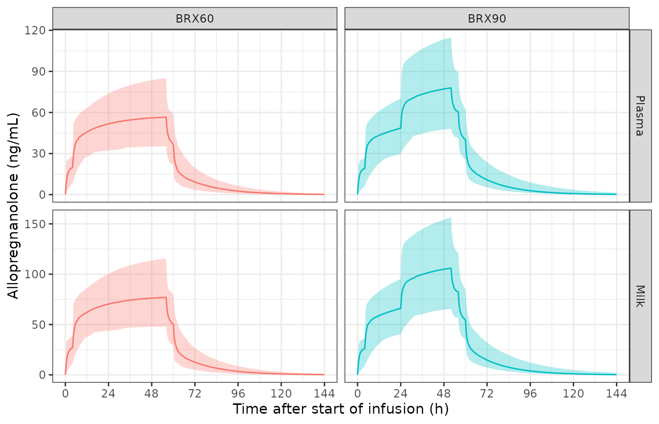
Replicates Figure 4a-d of Wald 2022: median and 95% prediction interval of allopregnanolone in plasma and breast milk for the BRX60 and BRX90 regimens (200 simulated subjects per regimen).
The paper’s Figure 4b plateau median at the end of the 90 ug/kg/h step is about 78 ng/mL (95% interval about 50-117 ng/mL), and Figure 4d shows the milk median at about 107 ng/mL. Figure 4a shows the BRX60 plateau median at about 54 ng/mL. These values were read from the published figure, so the check allows a 10% band on the medians.
plateau <- band_fig4 |>
  dplyr::filter((regimen == "BRX90" & time == 52) | (regimen == "BRX60" & time == 56)) |>
  dplyr::select(regimen, matrix, lo, med, hi)
plateau |>
  dplyr::rename("Regimen" = regimen, "Matrix" = matrix, "2.5th pct" = lo,
                "Median" = med, "97.5th pct" = hi) |>
knitr::kable(digits = 1, caption = "Simulated plateau concentrations (ng/mL) at 52 h (BRX90) and 56 h (BRX60).")| Regimen | Matrix | 2.5th pct | Median | 97.5th pct |
|---|---|---|---|---|
| BRX60 | Milk | 48.0 | 77.0 | 115.7 |
| BRX60 | Plasma | 35.3 | 56.6 | 85.1 |
| BRX90 | Milk | 65.4 | 106.0 | 156.3 |
| BRX90 | Plasma | 48.1 | 77.9 | 114.9 |
med_of <- function(reg, mat) plateau$med[plateau$regimen == reg & plateau$matrix == mat]
stopifnot(
  abs(med_of("BRX90", "Plasma") / 78 - 1) < 0.10,
  abs(med_of("BRX90", "Milk") / 107 - 1) < 0.10,
  abs(med_of("BRX60", "Plasma") / 54 - 1) < 0.10
)
The paper states that the model predicts milk allopregnanolone below 10 ng/mL 36 h after the end of the infusion (96 h) in 95% of subjects (section 3.5).
milk96_p95 <- sim_fig4 |>
  dplyr::filter(time == 96) |>
  dplyr::group_by(regimen) |>
  dplyr::summarise(p95_milk_ng_mL = quantile(Cmilk, 0.95), .groups = "drop")
milk96_p95 |>
  dplyr::rename("Regimen" = regimen, "95th pct milk conc (ng/mL)" = p95_milk_ng_mL) |>
  knitr::kable(digits = 2,
caption = "95th percentile of simulated milk concentration 36 h after the end of infusion.")| Regimen | 95th pct milk conc (ng/mL) |
|---|---|
| BRX60 | 8.16 |
| BRX90 | 9.47 |
# A 95th percentile of 200 subjects carries Monte Carlo noise of roughly 10%,
# so the check allows that margin above the paper's 10 ng/mL statement.
stopifnot(milk96_p95$p95_milk_ng_mL[milk96_p95$regimen == "BRX90"] < 12)
Relative infant dose (Table 4)
Table 4 of the paper derives the relative infant dose (RID) for the 24-48 h window of the BRX90 regimen (the day at the 90 ug/kg/h rate, a maternal dose of 2160 ug/kg/day): average milk concentration = milk AUC24-48 / 24 h, infant daily dose = average milk concentration x 150 mL/kg/day, and RID = infant dose / maternal dose.
conc_rid <- sim_fig4 |>
  dplyr::filter(regimen == "BRX90", !is.na(Cc)) |>
  dplyr::select(id, time, regimen, Plasma = Cc, Milk = Cmilk) |>
  tidyr::pivot_longer(c(Plasma, Milk), names_to = "matrix", values_to = "Cc")
dose_rid <- events_fig4 |>
  dplyr::filter(evid == 1, regimen == "BRX90", time == 0) |>
  dplyr::select(id, time, regimen, amt) |>
  tidyr::crossing(matrix = c("Plasma", "Milk"))

nca_rid <- PKNCA::pk.nca(PKNCA::PKNCAdata(
  PKNCA::PKNCAconc(conc_rid, Cc ~ time | regimen + matrix + id),
  PKNCA::PKNCAdose(dose_rid, amt ~ time | regimen + matrix + id, route = "intravascular"),
  intervals = data.frame(start = 24, end = 48, auclast = TRUE)
))

rid <- as.data.frame(nca_rid) |>
  dplyr::filter(PPTESTCD == "auclast") |>
  dplyr::select(id, matrix, PPORRES) |>
  tidyr::pivot_wider(names_from = matrix, values_from = PPORRES) |>
  dplyr::mutate(
    milk_avg = Milk / 24,
    infant_ug_kg_day = milk_avg * 150 / 1000,
    rid_pct = 100 * infant_ug_kg_day / 2160
  )

rid_summary <- data.frame(
  statistic = c("Minimum", "Median", "Maximum"),
  plasma_auc = c(min(rid$Plasma), median(rid$Plasma), max(rid$Plasma)),
  milk_auc = c(min(rid$Milk), median(rid$Milk), max(rid$Milk)),
  milk_avg = c(min(rid$milk_avg), median(rid$milk_avg), max(rid$milk_avg)),
  rid_pct = c(min(rid$rid_pct), median(rid$rid_pct), max(rid$rid_pct)),
  pub_plasma_auc = c(462, 1760, 3410),
  pub_milk_auc = c(628, 2394, 4638),
  pub_rid_pct = c(0.1818, 0.6926, 1.342)
)
rid_summary |>
  dplyr::rename(
    "Statistic" = statistic,
    "Plasma AUC24-48 (ng*h/mL)" = plasma_auc,
    "Milk AUC24-48 (ng*h/mL)" = milk_auc,
    "Average milk conc (ng/mL)" = milk_avg,
    "RID (%)" = rid_pct,
    "Published plasma AUC24-48" = pub_plasma_auc,
    "Published milk AUC24-48" = pub_milk_auc,
    "Published RID (%)" = pub_rid_pct
  ) |>
  knitr::kable(digits = c(0, 0, 0, 1, 3, 0, 0, 3),
caption = "Relative infant dose, BRX90, 24-48 h (simulated vs Table 4 of Wald 2022).")| Statistic | Plasma AUC24-48 (ng*h/mL) | Milk AUC24-48 (ng*h/mL) | Average milk conc (ng/mL) | RID (%) | Published plasma AUC24-48 | Published milk AUC24-48 | Published RID (%) |
|---|---|---|---|---|---|---|---|
| Minimum | 666 | 906 | 37.7 | 0.262 | 462 | 628 | 0.182 |
| Median | 1726 | 2347 | 97.8 | 0.679 | 1760 | 2394 | 0.693 |
| Maximum | 2782 | 3784 | 157.7 | 1.095 | 3410 | 4638 | 1.342 |
# The minimum and maximum depend on which subjects land in the tails, so
# only the medians are checked. Milk/plasma AUC is Kp = 1.36 by construction.
stopifnot(
  abs(median(rid$Plasma) / 1760 - 1) < 0.15,
  abs(median(rid$rid_pct) / 0.6926 - 1) < 0.15,
  abs(median(rid$Milk / rid$Plasma) - 1.36) < 1e-6
)
PKNCA validation against Table 3
Table 3 is a non-compartmental analysis of the observed plasma data of the 11 healthy lactating volunteers in 547-CLP-108 (BRX90). The replication samples a virtual 547-CLP-108 cohort (median weight 79.6 kg, range 60.4-128 kg; Table 1) at the study’s nominal plasma times (pre-infusion, 12, 24, 36, 48, 56, 60, 61, 62, 64 and 72 h; main text 2.2) and adds the proportional residual error, because Table 3 summarises observed concentrations: the observed Cmax is a maximum over noisy samples.
wt_108 <- draw_weights(n_arm, 79.6, 0.22, 60.4, 128)
t_108 <- c(0, 12, 24, 36, 48, 56, 60, 61, 62, 64, 72)
events_108 <- make_events(wt_108, "BRX90", t_108, id_offset = 1000L) |>
  dplyr::mutate(treatment = "BRX90 (547-CLP-108)")

sim_108 <- rxode2::rxSolve(
  mod, events = events_108, keep = c("treatment", "WT"),
  returnType = "data.frame", useLinCmt = FALSE
)

# `sim` is the plasma observation with residual error; floor at 0 so that a
# rare negative draw cannot enter the log-linear terminal-phase fit.
conc_108 <- sim_108 |>
  dplyr::mutate(Cc = pmax(sim, 0)) |>
  dplyr::filter(!is.na(Cc)) |>
  dplyr::select(id, time, treatment, Cc)
# Pre-infusion record: allopregnanolone below the assay LLOQ (main text 3.2).
conc_108 <- conc_108 |>
  dplyr::mutate(Cc = dplyr::if_else(time == 0, 0, Cc))

# One dose record per subject carrying the total 60-h amount, so PKNCA's
# clearance is total dose / AUC0-inf as in Table 3. The dose is intravenous
# (F = 1), so the "CL/F" label PKNCA attaches below is the systemic CL.
dose_108 <- events_108 |>
  dplyr::filter(evid == 1) |>
  dplyr::group_by(id, treatment) |>
  dplyr::summarise(amt = sum(amt) / 1000, time = 0, .groups = "drop")  # ug -> mg

intervals_108 <- data.frame(
  start = c(0, 0, 24),
  end = c(Inf, 60, 56),
  cmax = c(TRUE, FALSE, FALSE),
  tmax = c(TRUE, FALSE, FALSE),
  aucinf.obs = c(TRUE, FALSE, FALSE),
  half.life = c(TRUE, FALSE, FALSE),
  cl.obs = c(TRUE, FALSE, FALSE),
  auclast = c(FALSE, TRUE, TRUE),
  cav = c(FALSE, FALSE, TRUE)
)

nca_108 <- PKNCA::pk.nca(PKNCA::PKNCAdata(
  PKNCA::PKNCAconc(conc_108, Cc ~ time | treatment + id),
  PKNCA::PKNCAdose(dose_108, amt ~ time | treatment + id,
                   route = "intravascular", duration = 60),
  intervals = intervals_108
))
nca_long <- as.data.frame(nca_108) |>
  dplyr::filter(PPTESTCD %in% c("cmax", "tmax", "aucinf.obs", "half.life",
                                "cl.obs", "auclast", "cav")) |>
  dplyr::mutate(
    interval = dplyr::case_when(
      start == 0 & end == 60 ~ "0-60 h",
      start == 24 & end == 56 ~ "24-56 h",
      TRUE ~ "0-inf"
    ),
    # PKNCA clearance is mg / (ng*h/mL) = 1000 L/h; convert to L/h.
    PPORRES = dplyr::if_else(PPTESTCD == "cl.obs", PPORRES * 1000, PPORRES)
  )

# Table 3 reports geometric means (tmax: the paper's central value), so the
# simulated values are summarised the same way before comparison.
sim_summary <- nca_long |>
  dplyr::filter(!is.na(PPORRES), PPORRES > 0) |>
  dplyr::group_by(treatment, interval, PPTESTCD) |>
  dplyr::summarise(
    PPORRES = if (dplyr::first(PPTESTCD) == "tmax") median(PPORRES) else exp(mean(log(PPORRES))),
    .groups = "drop"
  )

published_108 <- data.frame(
  treatment = "BRX90 (547-CLP-108)",
  interval = c("0-inf", "0-inf", "0-inf", "0-inf", "0-inf",
               "0-60 h", "24-56 h", "24-56 h"),
  PPTESTCD = c("cmax", "tmax", "aucinf.obs", "half.life", "cl.obs",
               "auclast", "auclast", "cav"),
  PPORRES = c(89.7, 47.8, 3736.5, 11.3, 87.5, 3358.4, 2257.9, 70.6)
)

cmp_108 <- nlmixr2lib::ncaComparisonTable(
  simulated = sim_summary,
  reference = published_108,
  by = c("treatment", "interval"),
  units = c(cmax = "ng/mL", tmax = "h", aucinf.obs = "ng*h/mL",
            half.life = "h", cl.obs = "L/h", auclast = "ng*h/mL", cav = "ng/mL"),
  tolerance_pct = 20
)
cmp_108 |>
  dplyr::rename("Treatment" = treatment, "Interval" = interval) |>
knitr::kable(caption = "Plasma NCA: simulated 547-CLP-108 cohort vs Table 3 of Wald 2022 (geometric means; tmax median).")| NCA parameter | Treatment | Interval | Reference | Simulated | % diff |
|---|---|---|---|---|---|
| Cmax (ng/mL) | BRX90 (547-CLP-108) | 0-inf | 89.7 | 88 | -1.9% |
| Tmax (h) | BRX90 (547-CLP-108) | 0-inf | 47.8 | 48 | +0.4% |
| AUC0-∞ (obs) (ng*h/mL) | BRX90 (547-CLP-108) | 0-inf | 3740 | 3610 | -3.3% |
| AUClast (ng*h/mL) | BRX90 (547-CLP-108) | 0-60 h | 3360 | 3160 | -5.8% |
| AUClast (ng*h/mL) | BRX90 (547-CLP-108) | 24-56 h | 2260 | 2150 | -4.6% |
| t½ (h) | BRX90 (547-CLP-108) | 0-inf | 11.3 | 11 | -3.0% |
| CL/F (L/h) | BRX90 (547-CLP-108) | 0-inf | 87.5 | 96.3 | +10.0% |
| Cavg (ng/mL) | BRX90 (547-CLP-108) | 24-56 h | 70.6 | 67.3 | -4.7% |
if (!is.null(attr(cmp_108, "footnote"))) cat(attr(cmp_108, "footnote"), "\n")

pct_diff <- function(code, iv = "0-inf") {
  s <- sim_summary$PPORRES[sim_summary$PPTESTCD == code & sim_summary$interval == iv]
  r <- published_108$PPORRES[published_108$PPTESTCD == code & published_108$interval == iv]
  # A missing match would make the comparison below vacuously TRUE.
  stopifnot(length(s) == 1, length(r) == 1)
  100 * (s / r - 1)
}
# Geometric means of a 200-subject cohort; a mis-transcribed CL, volume or
# dose unit moves these by tens of percent.
stopifnot(
  abs(pct_diff("cmax")) < 15,
  abs(pct_diff("cav", "24-56 h")) < 15,
  abs(pct_diff("auclast", "0-60 h")) < 15,
  abs(pct_diff("auclast", "24-56 h")) < 15,
  abs(pct_diff("half.life")) < 20,
  abs(pct_diff("aucinf.obs")) < 15,
  abs(pct_diff("cl.obs")) < 15
)
Assumptions and deviations
- Residual error scale. ESM Table S1 prints the proportional residual variability as 0.272 without saying whether it is a standard deviation or a variance. The model uses it as an SD (27.2%). A simulation of the 547-CLP-108 design supports this reading. With SD 0.272 the geometric mean Cmax is about 88 ng/mL against the published 89.7, and the Cmax/Cavg ratio is about 1.30 against 1.27 (89.7/70.6). Reading 0.272 as a variance (SD 0.52) gives a Cmax of about 103 ng/mL and a ratio of about 1.55. The PKNCA comparison above repeats this check.
-
Milk residual error. Plasma and milk were fitted
simultaneously, but Table S1 lists a single proportional residual
variability. The same value is used for both matrices
(
propSdandpropSd_Cmilk). -
Partition coefficient. Kp (1.36) was estimated from
the 547-CLP-108 plasma and milk data and then held fixed when the plasma
model was updated with all five studies (Table S1 footnote). In the
model it is an ordinary
ini()value with no between-subject variability, as reported. Table S1 prints its “Relative SE (%)” as 0.235; with the 95% CI 0.858-2.16 this is the SE of log(Kp), not a percentage. - IIV. Only CL and V1 carry between-subject variability (Table S1), as an estimated covariance block (correlation 0.47).
- BRX60 schedule. The main text gives only the BRX90 schedule in full. For BRX60 the model uses 30 ug/kg/h for 0-4 h, 60 ug/kg/h for 4-56 h and 30 ug/kg/h for 56-60 h, which matches the steps visible in Figure 4a.
- Table 4 units. The column “Daily dose in milk, ug/kg/day” holds values in ng/kg/day (median 14,960 = 99.73 ng/mL x 150 mL/kg/day). Only with ng/kg/day does dividing by the maternal 2160 ug/kg/day give the tabulated RID of 0.69%.
- Weights. Virtual cohorts are log-normal, truncated to the observed ranges in Table 1: the pooled population for Figure 4 and Table 4, and the 547-CLP-108 arm for Table 3.
- Endogenous allopregnanolone. The model describes exogenous brexanolone only; there is no endogenous baseline. The paper notes that late milk samples are under-predicted because of undetected endogenous allopregnanolone (section 3.5).
- Errata. No erratum to the article was found (checked 2026-10-08).