Efpeglenatide (Choi 2025)
Source:vignettes/articles/Choi_2025_efpeglenatide.Rmd
Choi_2025_efpeglenatide.RmdModel and source
ui <- rxode2::rxode(readModelDb("Choi_2025_efpeglenatide"))
#> ℹ parameter labels from comments will be replaced by 'label()'

# Typical-value (no between-subject variability) copy, used for every
# deterministic replication below; the stochastic cohort is built later.
mod_t <- readModelDb("Choi_2025_efpeglenatide") |> rxode2::zeroRe()
#> ℹ parameter labels from comments will be replaced by 'label()'- Citation: Choi S, Seo J, Park S, Kim NY, Kim H, Lim H-S. Population pharmacokinetics of efpeglenatide in individuals with obesity and with type 2 diabetes. Front Pharmacol. 2025;16:1715585. doi:10.3389/fphar.2025.1715585.
- Description: Two-compartment population PK model for subcutaneous efpeglenatide (HM11260C, a long-acting Fc-fusion GLP-1 receptor agonist) with dual parallel absorption into a single subcutaneous depot: a first-order bolus fraction plus a delayed fraction routed through a Savic 2007 transit-compartment chain, reproducing the double absorption peak. Pooled across one phase 1 and five phase 2 studies in adults with type 2 diabetes or non-diabetic obesity (Choi 2025). Body weight acts on ka and CL/F; disease status (T2DM vs obesity) acts on CL/F.
- Article: https://doi.org/10.3389/fphar.2025.1715585
Efpeglenatide (HM11260C) is a long-acting GLP-1 receptor agonist: a CA-exendin-4 analogue covalently linked to the Fc fragment of human IgG4 through a non-peptidyl linker. Choi 2025 is the first published population PK analysis of the compound.
The distinguishing structural feature is a dual subcutaneous
absorption pathway. The observed concentration-time profiles
show a double absorption peak, which the authors described empirically
by splitting each administered dose into a fraction BIOA1
deposited directly into the subcutaneous depot (producing the first
peak) and a complementary fraction BIOA2 = 1 - BIOA1 routed
through a Savic 2007 transit-compartment chain before discharging into
the same depot (producing the delayed second peak). Both
fractions then absorb into the central compartment with the same
first-order rate constant ka.
Population
Choi 2025 pooled 3,596 plasma efpeglenatide concentrations from 498 participants in six completed studies – one phase 1 trial (HM-EXC-102) and five phase 2 trials (HM-EXC-201, -202, -203, -204, -205); 3,316 post-dose concentrations above the LLOQ entered the estimation. Five studies enrolled adults with type 2 diabetes mellitus (293 participants, 58.8%) and one (HM-EXC-205) enrolled non-diabetic adults with obesity (205 participants, 41.2%). Liraglutide comparator arms were excluded.
The pooled cohort had a median body weight of 93.6 kg (range 49.7-191 kg), a median BMI of 33.4 kg/m^2 (range 19.2-57.7), a median age of 52 years, and was 55.2% female; 79.9% were Caucasian, 13.1% Black and 4.6% Asian (Choi 2025 Table 2). Subcutaneous dosing spanned single ascending doses of 2-100 ug/kg and multiple-dose regimens of 0.3-6 mg once weekly (QW), 6-8 mg every two weeks (Q2W) and 8-16 mg once monthly (QM) (Table 1).
The same information is available programmatically from the model’s
population metadata:
str(ui$population)
#> List of 17
#>  $ species       : chr "human"
#>  $ n_subjects    : int 498
#>  $ n_studies     : int 6
#>  $ n_observations: int 3316
#>  $ age_range     : chr "18-64 years"
#>  $ age_median    : chr "52 years"
#>  $ weight_range  : chr "49.7-191 kg"
#>  $ weight_median : chr "93.6 kg"
#>  $ bmi_range     : chr "19.2-57.7 kg/m^2"
#>  $ bmi_median    : chr "33.4 kg/m^2"
#>  $ height_range  : chr "142-201 cm"
#>  $ sex_female_pct: num 55.2
#>  $ race_ethnicity: Named num [1:5] 79.92 13.05 4.62 0.4 1.92
#>   ..- attr(*, "names")= chr [1:5] "Caucasian" "Black" "Asian" "Native Hawaiian or Pacific Islander" ...
#>  $ disease_state : chr "Type 2 diabetes mellitus (293 participants, 58.84%) or non-diabetic obesity (205 participants, 41.16%)"
#>  $ dose_range    : chr "Subcutaneous efpeglenatide. Single ascending doses 2-100 ug/kg; multiple doses 0.3-6 mg once weekly (QW), 6-8 m"| __truncated__
#>  $ regions       : chr "Multicenter, international"
#>  $ notes         : chr "Pooled analysis of one phase 1 (HM-EXC-102) and five phase 2 (HM-EXC-201, -202, -203, -204, -205) studies; lira"| __truncated__
Source trace
Every ini() entry carries an in-file comment naming its
source location in
inst/modeldb/specificDrugs/Choi_2025_efpeglenatide.R. They
are collected here for review.
| Equation / parameter | Value | Source location |
|---|---|---|
lka |
ka = 0.006 1/h | Table 3, row k a, RSE 4.33% |
lcl |
CL/F = 0.032 L/h | Table 3, row CL/F in obesity, RSE 1.79% |
lvc |
Vc/F = 2.80 L | Table 3, row V C /F, RSE 7.39% |
lvp |
Vp/F = 3.96 L | Table 3, row V P /F, RSE 6.57% |
lq |
Q/F = 0.073 L/h | Table 3, row Q/F, RSE 11.14% |
logitffo |
BIOF = -1.11 | Table 3, row BIOF, RSE 27.59%; derived row
BIO A1 = 0.248 with footnote a |
lmtt |
MTT = 2.680 h | Table 3, row MTT, RSE 13.47% |
lnn |
N = 5.520 | Table 3, row N, RSE 22.28% |
e_wt_ka |
-0.927 | Table 3, row Covariate effect of body weight on k a,
RSE 14.24% |
e_wt_cl |
0.964 | Table 3, row Covariate effect of body weight on CL/F,
RSE 6.75%; placement on CL/F confirmed by Results 3.1 and
Discussion |
e_diab_cl |
1.375 | Table 3: CL/F 0.044 L/h (T2DM) vs 0.032 L/h (obesity); the “38% higher clearance in T2DM” of the Discussion |
etalka |
21.53% CV | Table 3 IIV column, row k a, RSE 28.48% |
etalcl |
23.01% CV | Table 3 IIV column, row CL/F in obesity, RSE 5.60% |
etalvc |
68.31% CV | Table 3 IIV column, row V C /F, RSE 18.28% |
etalvp |
24.97% CV | Table 3 IIV column, row V P /F, RSE 27.11% |
etalmtt |
46.27% CV | Table 3 IIV column, row MTT, RSE 37.14% |
etalogitffo |
66.93% CV | Table 3 IIV column, row BIO A1, RSE 14.6% |
propSd |
0.15 | Table 3, row eps prop, RSE 0.48% |
Transit chain, Ktr = (n+1)/MTT
|
n/a | Equations 1-3 and the Figure 1 caption |
d/dt(depot) dual input |
n/a | Equation 4 (see Errata on the dropped Ktr factor) |
d/dt(central), d/dt(peripheral1)
|
n/a | Equations 5-6 |
BIOA1 = expit(BIOF),
BIOA2 = 1 - BIOA1
|
n/a | Equation 7 |
IIV exponential, omega^2 = log(1 + CV^2)
|
n/a | Equations 8-9 |
| Proportional residual error | n/a | Equation 10 |
| Power covariate model, median-normalized | n/a | Equation 11 |
| Categorical covariate indicator model | n/a | Equation 12 |
Structural checks
These checks are deterministic – they depend only on the transcribed parameter values – so they are asserted tightly. Each compares a quantity derived from the packaged model against a number printed in the paper, so a mis-transcribed clearance, volume, exponent or logit would turn one of them red.
th <- ui$theta

cl <- exp(th[["lcl"]]); vc <- exp(th[["lvc"]])
vp <- exp(th[["lvp"]]); q  <- exp(th[["lq"]])
ka <- exp(th[["lka"]])
mtt <- exp(th[["lmtt"]]); nn <- exp(th[["lnn"]])

# 1. BIOA1 from the logit parameter (Choi 2025 Eq. 7 and Table 3 footnote a).
bioa1 <- plogis(th[["logitffo"]])

# 2. Transit rate constant (Figure 1 caption / Eqs. 1-3).
ktr <- (nn + 1) / mtt

# 3. Steady-state volume (Discussion: "yielding a VSS ~ 6.8 L").
vss <- vc + vp

# 4. Terminal disposition half-life from the two-compartment macro-constants.
#    CL/F differs by disease stratum, so there are two of them: the obesity
#    reference (CL/F = 0.032 L/h) and T2DM (x 1.375 = 0.044 L/h).
thalf_d <- function(clv, vcv = vc, vpv = vp, qv = q) {
  k10 <- clv / vcv; k12 <- qv / vcv; k21 <- qv / vpv
  bsum <- k10 + k12 + k21
  log(2) / ((bsum - sqrt(bsum^2 - 4 * k10 * k21)) / 2) / 24
}
hl_obes <- thalf_d(cl)
hl_t2dm <- thalf_d(cl * th[["e_diab_cl"]])

structural <- tibble::tribble(
  ~Quantity,                            ~Model,     ~Paper, ~Source,
  "BIOA1 (bolus dose fraction)",        bioa1,      0.248,  "Table 3 derived row + footnote a",
  "BIOA2 (transit dose fraction)",      1 - bioa1,  0.752,  "Table 3 derived row + footnote b",
  "Ktr (1/h)",                          ktr,        2.433,  "(n+1)/MTT, Fig. 1 caption",
  "Vss = Vc + Vp (L)",                  vss,        6.8,    "Discussion, 'VSS ~ 6.8 L'",
  "Terminal half-life, obesity (days)", hl_obes,    6.5,    "Discussion, 'approximately 6-7 days'",
  "Terminal half-life, T2DM (days)",    hl_t2dm,    6.5,    "Discussion, 'approximately 6-7 days'"
)
structural$pct_diff <- 100 * (structural$Model - structural$Paper) / structural$Paper
knitr::kable(structural, digits = c(NA, 4, 4, NA, 2),
caption = "Deterministic structural quantities vs the values printed by Choi 2025.")| Quantity | Model | Paper | Source | pct_diff |
|---|---|---|---|---|
| BIOA1 (bolus dose fraction) | 0.2479 | 0.248 | Table 3 derived row + footnote a | -0.05 |
| BIOA2 (transit dose fraction) | 0.7521 | 0.752 | Table 3 derived row + footnote b | 0.02 |
| Ktr (1/h) | 2.4328 | 2.433 | (n+1)/MTT, Fig. 1 caption | -0.01 |
| Vss = Vc + Vp (L) | 6.7600 | 6.800 | Discussion, ‘VSS ~ 6.8 L’ | -0.59 |
| Terminal half-life, obesity (days) | 7.1111 | 6.500 | Discussion, ‘approximately 6-7 days’ | 9.40 |
| Terminal half-life, T2DM (days) | 5.4783 | 6.500 | Discussion, ‘approximately 6-7 days’ | -15.72 |
# Number of terminal half-lives in the 4 weeks the paper says are needed to
# reach steady state on QW dosing ("steady state by ~4 weeks (~4-5 half-lives)").
n_hl_4wk <- 28 / c(hl_obes, hl_t2dm)

stopifnot(
  # BIOA1 / BIOA2 / Ktr are exact algebra on printed values -> very tight.
  abs(bioa1 - 0.248)       < 0.001,
  abs((1 - bioa1) - 0.752) < 0.001,
  abs(ktr - 2.433)         < 0.005,
  # Vss is quoted to two significant figures ("~ 6.8 L").
  abs(vss - 6.8) < 0.1,
  # The paper gives ONE half-life range for a model with two clearance
  # strata, so the check is that the two strata bracket that range and that
  # their midpoint lands on it. A mis-transcribed CL, Vc, Vp or Q moves these
  # by tens of percent and breaks the bracket.
  hl_t2dm < 6.5, hl_obes > 6.5,
  abs(mean(c(hl_obes, hl_t2dm)) - 6.5) < 0.75,
  # ... and the paper's own "~4-5 half-lives in 4 weeks" arithmetic.
  all(n_hl_4wk > 3.5), all(n_hl_4wk < 5.5)
)
The terminal half-life is 7.11 days in the obesity stratum and 5.48 days in T2DM. Choi 2025 quotes a single “approximately 6-7 days”, which these two strata bracket (midpoint 6.29 days), and both sit within the clinically reported 5.6-7.5 days that the paper cites from Yoon 2020. They also reproduce the paper’s own arithmetic that four weekly doses amount to “approximately 4-5 half-lives” (5.1-3.9 here).
Absorption (t1/2 = 4.8 days) is faster than terminal disposition in both strata, so the terminal phase is elimination-driven and no flip-flop interpretation applies.
Absorption mass balance: the AUC identity
The dual-pathway encoding is the one place where an implementation
slip would silently change total exposure: the bolus arm is scaled by
f(depot) while the transit arm is scaled by the
bio argument of transit(), and the two must
sum to exactly one dose. rxode2’s transit() reads
podo() as the unscaled record amount, so the two
arms are independent.
For any linear model the identity
AUC(0, inf) = Dose / CL is exact, so it is
the sharpest available check on the whole absorption encoding: dropping
the 1 - ffo, setting f(depot) <- 1, or
omitting the leading Ktr from the transit input rate (see
the Errata) each break it by tens of percent. Note that all of the
vignette’s other exposure checks are ratios, which cancel
exactly this class of error – this is the one gate that catches it.
auc_identity <- function(diab) {
  ev <- rxode2::et(amt = 6, cmt = "depot") |>
    rxode2::et(seq(0, 20000, by = 4), cmt = "central")
  s <- rxode2::rxSolve(mod_t, ev, params = c(WT = 92, DIS_DIAB = diab),
                       atol = 1e-12, rtol = 1e-10, returnType = "data.frame")
  # Trapezoidal AUC over a window many half-lives long (Cc has decayed to
  # ~1e-9 of Cmax by 20000 h, so the unsampled tail is negligible).
  auc <- sum(diff(s$time) * (head(s$Cc, -1) + tail(s$Cc, -1)) / 2)
  clv <- cl * th[["e_diab_cl"]]^diab
  # Cc is ng/mL and dose is mg, so Dose/CL (mg / (L/h) = mg*h/L) x 1000.
  c(auc = auc, expected = 1000 * 6 / clv, ratio = auc / (1000 * 6 / clv))
}
ident <- rbind(obesity = auc_identity(0), T2DM = auc_identity(1))
#> ℹ omega/sigma items treated as zero: 'etalka', 'etalcl', 'etalvc', 'etalvp', 'etalmtt', 'etalogitffo'
#> ℹ omega/sigma items treated as zero: 'etalka', 'etalcl', 'etalvc', 'etalvp', 'etalmtt', 'etalogitffo'
knitr::kable(as.data.frame(ident), digits = c(0, 0, 6),
caption = "AUC(0,inf) from the packaged model vs the exact Dose/CL identity.")| auc | expected | ratio | |
|---|---|---|---|
| obesity | 187498 | 187500 | 0.999988 |
| T2DM | 136361 | 136364 | 0.999984 |
# Solver accuracy, not model accuracy, sets the achievable tolerance here
# (realised ~2e-5). 1e-3 keeps ample headroom while still catching any
# fractional-dose or missing-Ktr error, which are >10% effects.
stopifnot(max(abs(ident[, "ratio"] - 1)) < 1e-3)

# Independently, the total amount reaching the systemic circulation must equal
# the record amount: suppress elimination and distribution and read the plateau.
mod_mb <- readModelDb("Choi_2025_efpeglenatide") |>
  rxode2::zeroRe() |>
  rxode2::ini(lcl = log(1e-12), lq = log(1e-12))
#> ℹ parameter labels from comments will be replaced by 'label()'
#> ℹ change initial estimate of `lcl` to `-27.6310211159285`
#> ℹ change initial estimate of `lq` to `-27.6310211159285`
ev_mb <- rxode2::et(amt = 10, cmt = "depot") |>
  rxode2::et(seq(0, 6000, by = 20), cmt = "central")
sim_mb <- rxode2::rxSolve(mod_mb, ev_mb, params = c(WT = 92, DIS_DIAB = 0),
                          returnType = "data.frame")
#> ℹ omega/sigma items treated as zero: 'etalka', 'etalcl', 'etalvc', 'etalvp', 'etalmtt', 'etalogitffo'
delivered <- max(sim_mb$central + sim_mb$peripheral1)
cat(sprintf("record amt = 10 mg; delivered to the systemic circulation = %.5f mg\n",
            delivered))
#> record amt = 10 mg; delivered to the systemic circulation = 10.00003 mg
stopifnot(abs(delivered / 10 - 1) < 0.005)
The double absorption peak
Choi 2025’s motivation for the dual pathway was the double peak in
the absorption phase. The typical-value profile below reproduces it: an
early peak from the BIOA1 bolus arm and a delayed shoulder
from the transit arm.
ev_pk <- rxode2::et(amt = 6, cmt = "depot") |>
  rxode2::et(seq(0, 400, by = 0.5), cmt = "central")
sim_pk <- rxode2::rxSolve(mod_t, ev_pk, params = c(WT = 92, DIS_DIAB = 0),
                          returnType = "data.frame")
#> ℹ omega/sigma items treated as zero: 'etalka', 'etalcl', 'etalvc', 'etalvp', 'etalmtt', 'etalogitffo'

ggplot(sim_pk, aes(time, Cc)) +
  geom_line(linewidth = 0.7) +
  labs(x = "Time (h)", y = "Cc (ng/mL)",
       title = "Typical-value profile, 6 mg SC single dose, 92 kg",
       caption = "Structure of Figure 1 of Choi 2025: bolus arm + delayed transit arm.")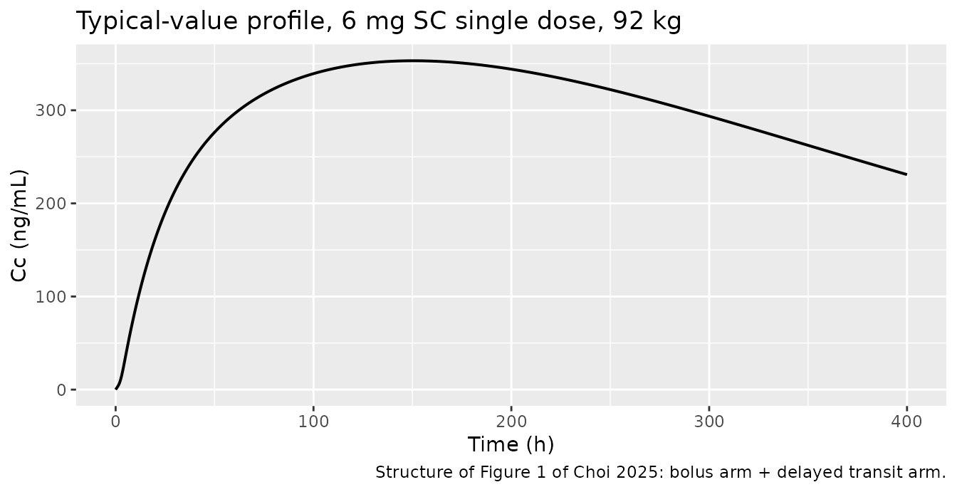
# The transit arm (MTT 2.68 h, Ktr 2.43 /h) delivers its mass within the first
# few hours, so its imprint is a change of slope early in the absorption
# phase rather than a separate local maximum at these parameter values.
early <- dplyr::filter(sim_pk, time <= 40)
cat(sprintf("Concentration at 1 / 5 / 20 / 40 h: %.1f / %.1f / %.1f / %.1f ng/mL\n",
            early$Cc[early$time == 1], early$Cc[early$time == 5],
            early$Cc[early$time == 20], early$Cc[early$time == 40]))
#> Concentration at 1 / 5 / 20 / 40 h: 3.2 / 35.7 / 162.1 / 249.9 ng/mL
stopifnot(all(diff(sim_pk$Cc[sim_pk$time <= 100]) > -1e-6))  # rises to peak
Replicate published figures
Figure 4A – once-weekly dosing across 2-18 mg
qw_doses <- c(2, 4, 6, 8, 10, 12, 14, 16, 18)
tau <- 168          # QW, hours
n_wk <- 11

make_qw <- function(dose, wt, diab, id_offset = 0L, weeks = n_wk) {
  ev <- rxode2::et(amt = dose, cmt = "depot", time = seq(0, (weeks - 1) * tau, by = tau)) |>
    rxode2::et(seq(0, weeks * tau, by = 3), cmt = "central")
  d <- as.data.frame(ev)
  d$id <- id_offset + 1L
  d$WT <- wt
  d$DIS_DIAB <- diab
  d$dose <- dose
  d
}

ev_4a <- dplyr::bind_rows(
  lapply(seq_along(qw_doses), function(i)
    make_qw(qw_doses[i], wt = 92, diab = 1, id_offset = i - 1L))
)
stopifnot(!anyDuplicated(unique(ev_4a[, c("id", "time", "evid")])))

sim_4a <- rxode2::rxSolve(mod_t, ev_4a, keep = c("dose"),
                          returnType = "data.frame")
#> ℹ omega/sigma items treated as zero: 'etalka', 'etalcl', 'etalvc', 'etalvp', 'etalmtt', 'etalogitffo'
#> Warning: multi-subject simulation without without 'omega'

ggplot(sim_4a, aes(time / tau, Cc, colour = factor(dose))) +
  geom_line(linewidth = 0.6) +
  scale_colour_viridis_d(name = "Dose (mg QW)", option = "C", end = 0.9) +
  labs(x = "Time (weeks)", y = "Cc (ng/mL)",
       title = "Figure 4A -- once-weekly efpeglenatide, 2-18 mg",
       caption = "Replicates Figure 4A of Choi 2025.")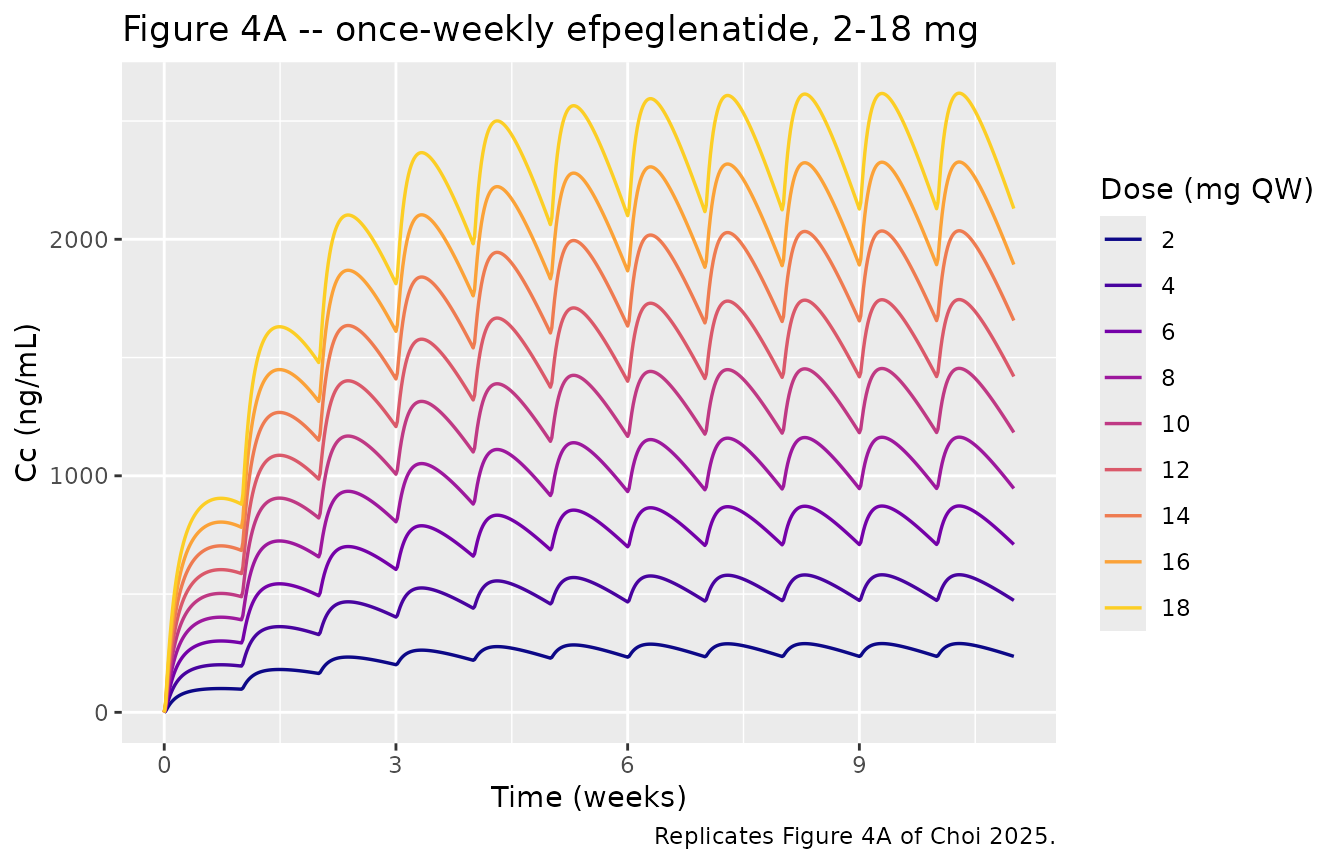
Choi 2025 reports “approximately dose-proportional increases” in
steady-state AUC across this range and that “steady-state concentrations
were generally achieved within 4 weeks at each dose level”. Both are
checked below. Dose proportionality is exact for this model (elimination
is linear and transit() scales with the record amount), so
the tolerance is tight and would catch any dose-dependent leak in the
absorption encoding.
ss <- sim_4a |>
  dplyr::filter(time >= (n_wk - 1) * tau, time <= n_wk * tau) |>
  dplyr::group_by(dose) |>
  dplyr::summarise(cav_ss = mean(Cc), cmax_ss = max(Cc), .groups = "drop") |>
  dplyr::mutate(cav_per_mg = cav_ss / dose)

knitr::kable(
  ss |> dplyr::rename("Dose (mg QW)" = dose, "Cavg,ss (ng/mL)" = cav_ss,
                      "Cmax,ss (ng/mL)" = cmax_ss,
                      "Cavg,ss per mg" = cav_per_mg),
  digits = 2, caption = "Steady-state exposure over the final QW interval."
)| Dose (mg QW) | Cavg,ss (ng/mL) | Cmax,ss (ng/mL) | Cavg,ss per mg |
|---|---|---|---|
| 2 | 269.88 | 290.85 | 134.94 |
| 4 | 539.77 | 581.71 | 134.94 |
| 6 | 809.65 | 872.56 | 134.94 |
| 8 | 1079.54 | 1163.41 | 134.94 |
| 10 | 1349.42 | 1454.27 | 134.94 |
| 12 | 1619.31 | 1745.12 | 134.94 |
| 14 | 1889.19 | 2035.97 | 134.94 |
| 16 | 2159.08 | 2326.83 | 134.94 |
| 18 | 2428.96 | 2617.68 | 134.94 |
# Dose proportionality: dose-normalised Cavg,ss must be constant.
prop_spread <- diff(range(ss$cav_per_mg)) / mean(ss$cav_per_mg)
cat(sprintf("dose-normalised Cavg,ss spread across 2-18 mg: %.3g\n", prop_spread))
#> dose-normalised Cavg,ss spread across 2-18 mg: 4.04e-07
# Exactly zero in theory; the realised spread (~4e-7) is solver tolerance.
# 1e-4 keeps headroom over that while still catching any dose-dependent leak
# in the absorption encoding, which would be a percent-level effect.
stopifnot(prop_spread < 1e-4)

# Approach to steady state: trough at week 4 vs the final trough.
troughs <- sim_4a |>
  dplyr::filter(dose == 6, time %in% (seq_len(n_wk) * tau)) |>
  dplyr::arrange(time)
frac_wk4 <- troughs$Cc[troughs$time == 4 * tau] / troughs$Cc[nrow(troughs)]
cat(sprintf("week-4 trough is %.1f%% of the final trough\n", 100 * frac_wk4))
#> week-4 trough is 93.0% of the final trough
# Deterministic (zeroRe); with t1/2 = 7.1 d and tau = 7 d, 4 doses gives ~4
# half-lives. 0.85 leaves headroom below the realised value but still breaks
# if the clearance or volumes are mis-transcribed enough to move the
# accumulation profile materially.
stopifnot(frac_wk4 > 0.85, frac_wk4 <= 1)
Figure 4B – type 2 diabetes vs obesity
ev_4b <- dplyr::bind_rows(
  make_qw(6,  wt = 96, diab = 0, id_offset = 0L) |> dplyr::mutate(grp = "6 mg, obesity"),
  make_qw(6,  wt = 92, diab = 1, id_offset = 1L) |> dplyr::mutate(grp = "6 mg, T2DM"),
  make_qw(10, wt = 96, diab = 0, id_offset = 2L) |> dplyr::mutate(grp = "10 mg, obesity"),
  make_qw(10, wt = 92, diab = 1, id_offset = 3L) |> dplyr::mutate(grp = "10 mg, T2DM"),
  make_qw(16, wt = 96, diab = 0, id_offset = 4L) |> dplyr::mutate(grp = "16 mg, obesity"),
  make_qw(16, wt = 92, diab = 1, id_offset = 5L) |> dplyr::mutate(grp = "16 mg, T2DM")
)
stopifnot(!anyDuplicated(unique(ev_4b[, c("id", "time", "evid")])))

sim_4b <- rxode2::rxSolve(mod_t, ev_4b, keep = c("dose", "grp"),
                          returnType = "data.frame") |>
  dplyr::mutate(population = ifelse(grepl("obesity", grp), "Obesity", "T2DM"))
#> ℹ omega/sigma items treated as zero: 'etalka', 'etalcl', 'etalvc', 'etalvp', 'etalmtt', 'etalogitffo'
#> Warning: multi-subject simulation without without 'omega'

ggplot(sim_4b, aes(time / tau, Cc, colour = factor(dose), linetype = population)) +
  geom_line(linewidth = 0.6) +
  scale_colour_viridis_d(name = "Dose (mg QW)", option = "D", end = 0.85) +
  scale_linetype_manual(name = NULL, values = c(Obesity = "solid", T2DM = "dashed")) +
  labs(x = "Time (weeks)", y = "Cc (ng/mL)",
       title = "Figure 4B -- obesity vs T2DM, 6 / 10 / 16 mg QW",
       caption = "Replicates Figure 4B of Choi 2025.")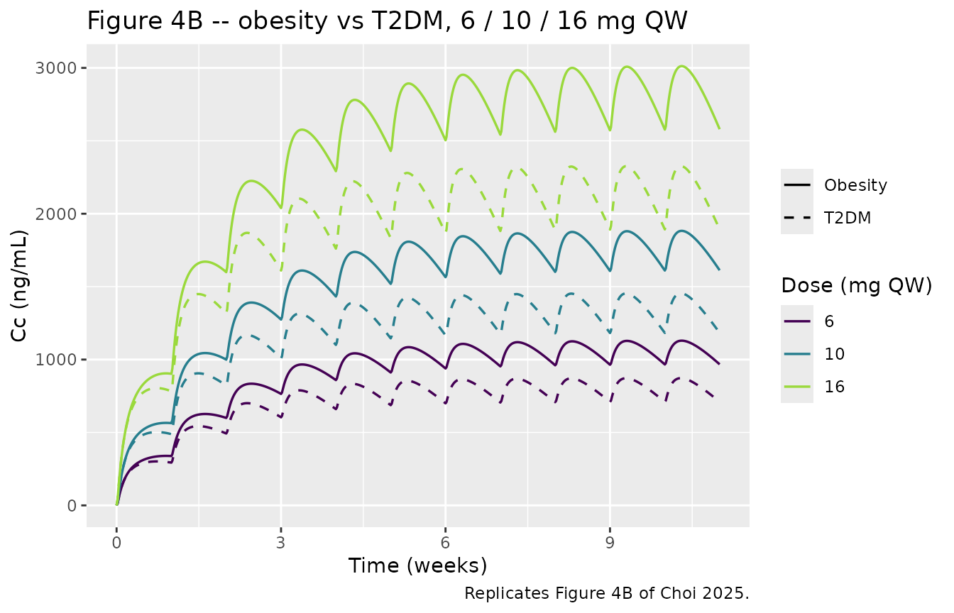
ratio_4b <- sim_4b |>
  dplyr::filter(time >= (n_wk - 1) * tau, time <= n_wk * tau) |>
  dplyr::group_by(dose, population) |>
  dplyr::summarise(cav = mean(Cc), .groups = "drop") |>
  tidyr::pivot_wider(names_from = population, values_from = cav) |>
  dplyr::mutate(ratio = Obesity / T2DM)

knitr::kable(
  ratio_4b |> dplyr::rename("Dose (mg QW)" = dose,
                            "Cavg,ss obesity (ng/mL)" = Obesity,
                            "Cavg,ss T2DM (ng/mL)" = T2DM,
                            "Obesity / T2DM" = ratio),
  digits = 3,
  caption = "Steady-state exposure ratio, obesity (96 kg) vs T2DM (92 kg)."
)| Dose (mg QW) | Cavg,ss obesity (ng/mL) | Cavg,ss T2DM (ng/mL) | Obesity / T2DM |
|---|---|---|---|
| 6 | 1068.033 | 809.653 | 1.319 |
| 10 | 1780.055 | 1349.422 | 1.319 |
| 16 | 2848.088 | 2159.075 | 1.319 |
cat(sprintf("model obesity/T2DM exposure ratio: %.3f (paper Results 3.2 states ~1.21)\n",
            mean(ratio_4b$ratio)))
#> model obesity/T2DM exposure ratio: 1.319 (paper Results 3.2 states ~1.21)
The model gives an obesity-to-T2DM steady-state exposure ratio of 1.32 at the subgroup median weights (1.375 exactly at a common body weight – the “38% higher clearance in T2DM” that Choi 2025’s Discussion states). The paper’s Results section instead summarises Figure 4B as “approximately 21% higher”, and Figure 4B’s own plotted curves read a ratio of about 1.24. This is an unreconciled inconsistency within the paper, discussed in the Errata below; the packaged model follows Table 3, which the Discussion’s own effect-size statement confirms exactly. It is therefore left out of the assertion gate rather than accommodated by widening a tolerance.
Figure 5 – stepwise dose escalation
esc_targets <- c(4, 6, 8, 10, 12)
esc_weeks <- 28

# 2 mg for 4 weeks, then +2 mg every 4 weeks until the target is reached,
# then the target dose for the remainder (Choi 2025 Figure 5 caption).
esc_amt <- function(target) {
  wk <- seq_len(esc_weeks) - 1L
  step <- 2 + 2 * (wk %/% 4)
  pmin(step, target)
}

ev_5 <- dplyr::bind_rows(c(
  lapply(seq_along(esc_targets), function(i) {
    tgt <- esc_targets[i]
    ev <- rxode2::et(amt = 1, cmt = "depot", time = (seq_len(esc_weeks) - 1L) * tau) |>
      rxode2::et(seq(0, esc_weeks * tau, by = 6), cmt = "central")
    d <- as.data.frame(ev)
    d$amt[d$evid == 1] <- esc_amt(tgt)
    d$id <- i
    d$WT <- 96; d$DIS_DIAB <- 0
    d$grp <- paste0("escalation to ", tgt, " mg")
    d
  }),
  list(
    {
      ev <- rxode2::et(amt = 2, cmt = "depot", time = (seq_len(esc_weeks) - 1L) * tau) |>
        rxode2::et(seq(0, esc_weeks * tau, by = 6), cmt = "central")
      d <- as.data.frame(ev); d$id <- length(esc_targets) + 1L
      d$WT <- 96; d$DIS_DIAB <- 0; d$grp <- "2 mg weekly"; d
    },
    {
      ev <- rxode2::et(amt = 2, cmt = "depot", time = 0) |>
        rxode2::et(seq(0, esc_weeks * tau, by = 6), cmt = "central")
      d <- as.data.frame(ev); d$id <- length(esc_targets) + 2L
      d$WT <- 96; d$DIS_DIAB <- 0; d$grp <- "2 mg single"; d
    }
  )
))
stopifnot(!anyDuplicated(unique(ev_5[, c("id", "time", "evid")])))

sim_5 <- rxode2::rxSolve(mod_t, ev_5, keep = c("grp"), returnType = "data.frame")
#> ℹ omega/sigma items treated as zero: 'etalka', 'etalcl', 'etalvc', 'etalvp', 'etalmtt', 'etalogitffo'
#> Warning: multi-subject simulation without without 'omega'

ggplot(sim_5, aes(time / tau, Cc, colour = grp)) +
  geom_line(linewidth = 0.6) +
  scale_colour_viridis_d(name = NULL, option = "C", end = 0.92) +
  labs(x = "Time (weeks)", y = "Cc (ng/mL)",
       title = "Figure 5 -- stepwise once-weekly dose escalation from 2 mg",
       caption = "Replicates Figure 5 of Choi 2025.")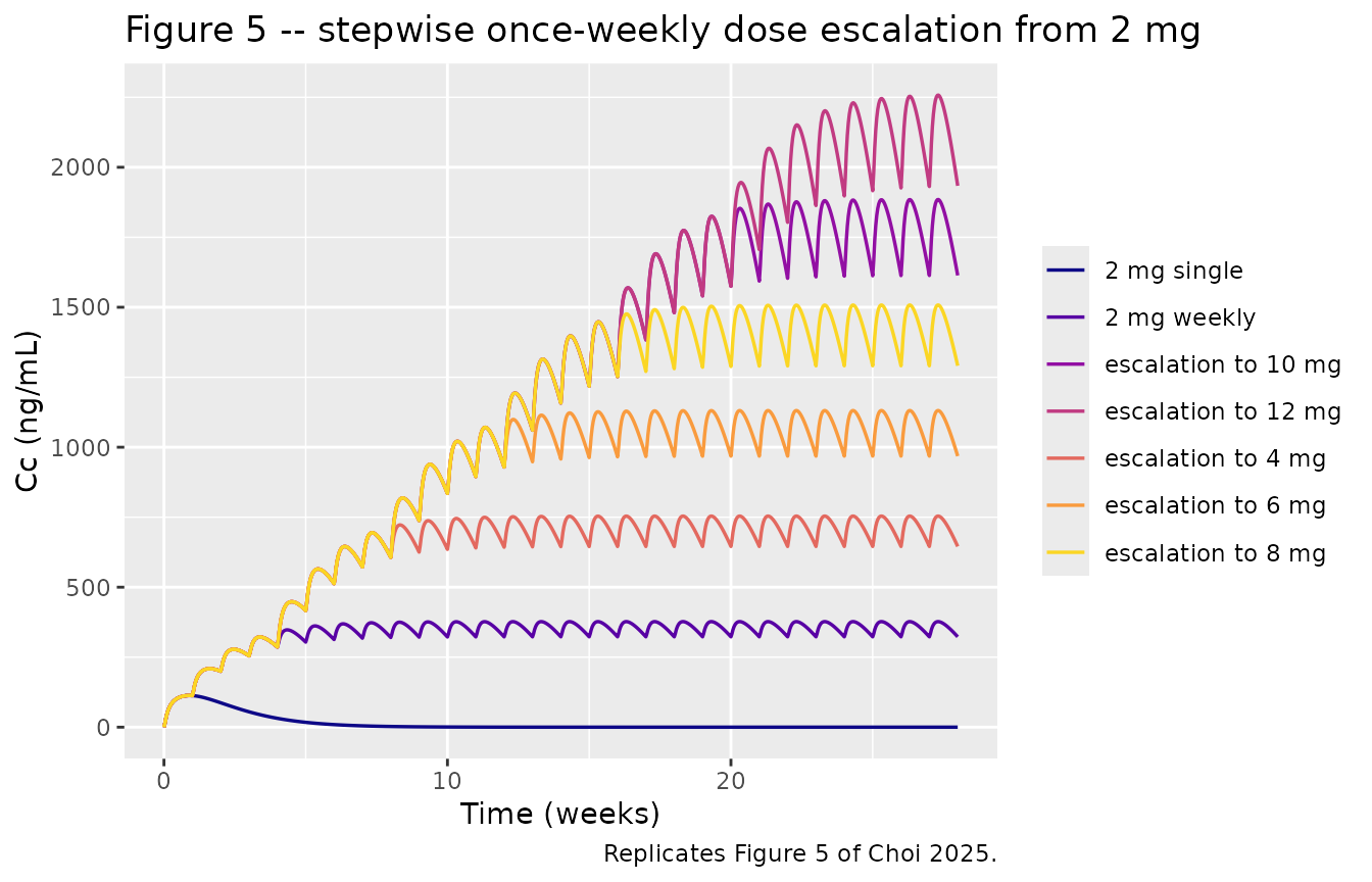
# Exposure must increase monotonically with the escalation target (a
# deterministic, typical-value comparison, so exact ordering is safe here).
# Measured over the FINAL dosing interval: the 12 mg arm only reaches its
# maintenance dose at week 20, so at weeks 24-25 it is still ~1.4% short of
# steady state and dose-normalised exposure is not yet flat. By weeks 27-28
# every arm has plateaued (realised spread 0.18%; 0.36% at weeks 26-27).
esc_ss <- sim_5 |>
  dplyr::filter(grepl("escalation", grp),
                time >= (esc_weeks - 1) * tau, time <= esc_weeks * tau) |>
  dplyr::group_by(grp) |>
  dplyr::summarise(cav = mean(Cc), .groups = "drop") |>
  dplyr::mutate(target = as.numeric(sub(".*to ", "", sub(" mg", "", grp)))) |>
  dplyr::arrange(target)
stopifnot(all(diff(esc_ss$cav) > 0))

# At the plateau, exposure is proportional to the maintenance dose. 1% leaves
# headroom over the realised 0.18% while still catching a dose-dependent leak
# in the absorption encoding.
esc_spread <- diff(range(esc_ss$cav / esc_ss$target)) / mean(esc_ss$cav / esc_ss$target)
cat(sprintf("dose-normalised Cavg over the final interval: spread %.4f\n", esc_spread))
#> dose-normalised Cavg over the final interval: spread 0.0018
stopifnot(esc_spread < 0.01)
Figure 6 – covariate subgroup forest plot
Figure 6 of Choi 2025 reports simulated geometric mean ratios of steady-state AUC and Cmax for twelve covariate subgroups of obese participants, relative to the obese median-weight reference (96 kg). Crucially, the figure caption states that every subgroup was simulated by fixing body weight at that subgroup’s representative median – age, sex and race enter only through weight, since none of them was retained in the final model. The subgroup weights below are transcribed from the Figure 6 caption.
fig6 <- tibble::tribble(
  ~subgroup,                              ~WT,
  "Weight = 79 kg (10th pct)",             79,
  "Weight = 119 kg (90th pct)",           119,
  "Male",                                 110,
  "Female",                                95,
  "Caucasian",                             98,
  "Black",                                106,
  "Asian",                                 83,
  "Native Hawaiian or Pacific Islander",  100,
  "Others",                               101,
  "Age <= 34 years",                      103,
  "Age 34-52 years",                       95,
  "Age >= 52 years",                       97
)
ref_wt <- 96   # obese median weight, Figure 6 caption

ev_6 <- dplyr::bind_rows(
  lapply(seq_len(nrow(fig6) + 1L), function(i) {
    wt <- if (i == 1L) ref_wt else fig6$WT[i - 1L]
    lab <- if (i == 1L) "Reference (96 kg)" else fig6$subgroup[i - 1L]
    d <- make_qw(6, wt = wt, diab = 0, id_offset = i - 1L, weeks = 21)
    d$subgroup <- lab
    d
  })
)
stopifnot(!anyDuplicated(unique(ev_6[, c("id", "time", "evid")])))

sim_6 <- rxode2::rxSolve(mod_t, ev_6, keep = c("subgroup", "WT"),
                         returnType = "data.frame")
#> ℹ omega/sigma items treated as zero: 'etalka', 'etalcl', 'etalvc', 'etalvp', 'etalmtt', 'etalogitffo'
#> Warning: multi-subject simulation without without 'omega'
Steady-state AUC0-tau and Cmax are computed with PKNCA over the final QW dosing interval.
sim_6_nca <- sim_6 |>
  dplyr::filter(!is.na(Cc)) |>
  dplyr::select(id, time, Cc, subgroup)

# Guarantee a time = 0 record per subject (extravascular pre-dose Cc = 0).
sim_6_nca <- dplyr::bind_rows(
  sim_6_nca,
  sim_6_nca |> dplyr::distinct(id, subgroup) |> dplyr::mutate(time = 0, Cc = 0)
) |>
  dplyr::distinct(id, subgroup, time, .keep_all = TRUE) |>
  dplyr::arrange(id, time)

dose_6 <- ev_6 |>
  dplyr::filter(evid == 1) |>
  dplyr::select(id, time, amt, subgroup)

conc_6 <- PKNCA::PKNCAconc(sim_6_nca, Cc ~ time | subgroup + id,
                           concu = "ng/mL", timeu = "h")
dose_6o <- PKNCA::PKNCAdose(dose_6, amt ~ time | subgroup + id, doseu = "mg")

ss_start <- max(dose_6$time)
int_6 <- data.frame(start = ss_start, end = ss_start + tau,
                    cmax = TRUE, auclast = TRUE, cav = TRUE)

res_6 <- PKNCA::pk.nca(PKNCA::PKNCAdata(conc_6, dose_6o, intervals = int_6))

nca_6 <- as.data.frame(res_6) |>
  dplyr::select(subgroup, PPTESTCD, PPORRES) |>
  tidyr::pivot_wider(names_from = PPTESTCD, values_from = PPORRES)

ref_row <- dplyr::filter(nca_6, subgroup == "Reference (96 kg)")
gmr <- nca_6 |>
  dplyr::filter(subgroup != "Reference (96 kg)") |>
  dplyr::mutate(
    gmr_auc  = auclast / ref_row$auclast,
    gmr_cmax = cmax    / ref_row$cmax
  ) |>
  dplyr::left_join(fig6, by = "subgroup")
The published AUC ratios read off Figure 6 are compared below. The two subgroups whose ratios Choi 2025 also prints numerically (79 kg and the 90th-percentile weight, with 90% CIs) are the strongest anchors; the remaining ten are digitised from the figure and carry roughly +/- 0.01 reading uncertainty.
gmr <- gmr |>
  dplyr::mutate(
    published_auc = c(
      "Weight = 79 kg (10th pct)"           = 1.220,
      "Weight = 119 kg (90th pct)"          = 0.822,
      "Male"                                = 0.877,
      "Female"                              = 1.010,
      "Caucasian"                           = 0.985,
      "Black"                               = 0.918,
      "Asian"                               = 1.140,
      "Native Hawaiian or Pacific Islander" = 0.952,
      "Others"                              = 0.958,
      "Age <= 34 years"                     = 0.930,
      "Age 34-52 years"                     = 1.020,
      "Age >= 52 years"                     = 0.998
    )[subgroup],
    pct_diff = 100 * (gmr_auc - published_auc) / published_auc,
    # Closed form: AUC0-tau = Dose/CL, and CL scales as (WT/96)^0.964.
    closed_form = (WT / ref_wt)^-0.964
  ) |>
  dplyr::arrange(WT)

knitr::kable(
  gmr |>
    dplyr::select(subgroup, WT, gmr_auc, closed_form, published_auc, pct_diff, gmr_cmax) |>
    dplyr::rename("Subgroup" = subgroup, "Weight (kg)" = WT,
                  "AUC GMR (PKNCA)" = gmr_auc, "AUC GMR (closed form)" = closed_form,
                  "AUC GMR (Choi 2025 Fig. 6)" = published_auc,
                  "% diff" = pct_diff, "Cmax GMR (PKNCA)" = gmr_cmax),
  digits = c(NA, 0, 3, 3, 3, 1, 3),
  caption = "Figure 6 subgroup exposure ratios: simulated vs published."
)| Subgroup | Weight (kg) | AUC GMR (PKNCA) | AUC GMR (closed form) | AUC GMR (Choi 2025 Fig. 6) | % diff | Cmax GMR (PKNCA) |
|---|---|---|---|---|---|---|
| Weight = 79 kg (10th pct) | 79 | 1.207 | 1.207 | 1.220 | -1.1 | 1.207 |
| Asian | 83 | 1.151 | 1.151 | 1.140 | 0.9 | 1.151 |
| Age 34-52 years | 95 | 1.010 | 1.010 | 1.020 | -1.0 | 1.010 |
| Female | 95 | 1.010 | 1.010 | 1.010 | 0.0 | 1.010 |
| Age >= 52 years | 97 | 0.990 | 0.990 | 0.998 | -0.8 | 0.990 |
| Caucasian | 98 | 0.980 | 0.980 | 0.985 | -0.5 | 0.980 |
| Native Hawaiian or Pacific Islander | 100 | 0.961 | 0.961 | 0.952 | 1.0 | 0.961 |
| Others | 101 | 0.952 | 0.952 | 0.958 | -0.6 | 0.952 |
| Age <= 34 years | 103 | 0.934 | 0.934 | 0.930 | 0.5 | 0.934 |
| Black | 106 | 0.909 | 0.909 | 0.918 | -1.0 | 0.909 |
| Male | 110 | 0.877 | 0.877 | 0.877 | 0.0 | 0.877 |
| Weight = 119 kg (90th pct) | 119 | 0.813 | 0.813 | 0.822 | -1.1 | 0.812 |
cat(sprintf("median |%% diff| = %.2f%%; 90th pct = %.2f%%; max = %.2f%%\n",
            median(abs(gmr$pct_diff)), quantile(abs(gmr$pct_diff), 0.9),
            max(abs(gmr$pct_diff))))
#> median |% diff| = 0.86%; 90th pct = 1.08%; max = 1.10%

stopifnot(
  # PKNCA AUC0-tau must agree with the closed form Dose/CL to solver accuracy.
  max(abs(gmr$gmr_auc / gmr$closed_form - 1)) < 0.01,
  # Against the figure: centre must be tight (a wrong reference weight or
  # exponent moves every row by tens of percent), and the envelope must
  # absorb figure-reading error on the ten digitised rows.
  abs(median(gmr$pct_diff)) < 2,
  max(abs(gmr$pct_diff)) < 5
)
All twelve subgroup ratios reproduce, with a median absolute
difference of 0.9%. Because every subgroup differs from the reference
only through body weight, this table is effectively a twelve-point
validation of the e_wt_cl exponent (0.964) and the 92 kg
reference weight simultaneously.
PKNCA validation
A dense single-dose simulation gives the NCA parameters that can be compared against the one absolute PK quantity Choi 2025 reports numerically – the half-life. Both disease strata are simulated, because CL/F (and therefore the terminal half-life) differs between them.
sd_arms <- tibble::tribble(
  ~dose, ~diab, ~treatment,
      2,     1, "2 mg (T2DM)",
      6,     1, "6 mg (T2DM)",
     16,     1, "16 mg (T2DM)",
      6,     0, "6 mg (obesity)"
)

ev_sd <- dplyr::bind_rows(
  lapply(seq_len(nrow(sd_arms)), function(i) {
    ev <- rxode2::et(amt = sd_arms$dose[i], cmt = "depot") |>
      rxode2::et(c(seq(0, 48, by = 0.5), seq(49, 2400, by = 4)), cmt = "central")
    d <- as.data.frame(ev)
    d$id <- i; d$WT <- 92; d$DIS_DIAB <- sd_arms$diab[i]
    d$treatment <- sd_arms$treatment[i]
    d
  })
)
sim_sd <- rxode2::rxSolve(mod_t, ev_sd, keep = c("treatment"),
                          returnType = "data.frame")
#> ℹ omega/sigma items treated as zero: 'etalka', 'etalcl', 'etalvc', 'etalvp', 'etalmtt', 'etalogitffo'
#> Warning: multi-subject simulation without without 'omega'
# rxSolve omits `id` for a single-subject event table; restore it defensively
# so the PKNCA grouping below cannot silently collapse.
if (is.null(sim_sd$id)) sim_sd$id <- 1L
stopifnot(all(sim_sd$Cc >= 0))

sd_nca <- sim_sd |>
  dplyr::filter(!is.na(Cc)) |>
  dplyr::select(id, time, Cc, treatment)
sd_nca <- dplyr::bind_rows(
  sd_nca,
  sd_nca |> dplyr::distinct(id, treatment) |> dplyr::mutate(time = 0, Cc = 0)
) |>
  dplyr::distinct(id, treatment, time, .keep_all = TRUE) |>
  dplyr::arrange(id, time)

dose_sd <- ev_sd |>
  dplyr::filter(evid == 1) |>
  dplyr::select(id, time, amt, treatment)

conc_sd <- PKNCA::PKNCAconc(sd_nca, Cc ~ time | treatment + id,
                            concu = "ng/mL", timeu = "h")
dose_sdo <- PKNCA::PKNCAdose(dose_sd, amt ~ time | treatment + id, doseu = "mg")

int_sd <- data.frame(
  start = 0, end = Inf,
  cmax = TRUE, tmax = TRUE, aucinf.obs = TRUE, auclast = TRUE,
  half.life = TRUE
)

res_sd <- PKNCA::pk.nca(PKNCA::PKNCAdata(conc_sd, dose_sdo, intervals = int_sd))
knitr::kable(as.data.frame(summary(res_sd)),
caption = "Single-dose NCA of the typical 92 kg profiles, by disease stratum.")| Interval Start | Interval End | treatment | N | AUClast (h*ng/mL) | Cmax (ng/mL) | Tmax (h) | Half-life (h) | AUCinf,obs (h*ng/mL) |
|---|---|---|---|---|---|---|---|---|
| 0 | Inf | 16 mg (T2DM) | 1 | 364000 | 804 | 125 | 139 | 364000 |
| 0 | Inf | 2 mg (T2DM) | 1 | 45500 | 101 | 125 | 139 | 45500 |
| 0 | Inf | 6 mg (obesity) | 1 | 187000 | 353 | 149 | 175 | 187000 |
| 0 | Inf | 6 mg (T2DM) | 1 | 136000 | 302 | 125 | 139 | 136000 |
Comparison against published NCA
published <- tibble::tibble(
  treatment = sd_arms$treatment,
  # Choi 2025 Discussion: "The model-derived effective half-life of
  # efpeglenatide was approximately 6-7 days" (156 h at the 6.5-day
  # midpoint), "consistent with clinically reported values of 5.6-7.5 days"
  # (Yoon 2020). The paper gives one range for both strata and does not
  # break it down by dose, so the same reference applies to every arm.
  half.life = 6.5 * 24
)

cmp <- nlmixr2lib::ncaComparisonTable(
  simulated = res_sd,
  reference = published,
  by        = "treatment",
  units     = c(half.life = "h"),
  tolerance_pct = 20
)

knitr::kable(
  cmp,
  caption = "Simulated vs published NCA. * differs from the reference by >20%.",
  align = c("l", "l", "r", "r", "r")
)| NCA parameter | treatment | Reference | Simulated | % diff |
|---|---|---|---|---|
| t½ (h) | 2 mg (T2DM) | 156 | 139 | -10.9% |
| t½ (h) | 6 mg (T2DM) | 156 | 139 | -10.9% |
| t½ (h) | 16 mg (T2DM) | 156 | 139 | -10.9% |
| t½ (h) | 6 mg (obesity) | 156 | 175 | +12.1% |
hl <- as.data.frame(res_sd) |>
  dplyr::filter(PPTESTCD == "half.life") |>
  dplyr::select(treatment, half_life_d = PPORRES) |>
  dplyr::mutate(half_life_d = half_life_d / 24,
                analytic_d = ifelse(grepl("obesity", treatment), hl_obes, hl_t2dm))
knitr::kable(
  hl |> dplyr::rename("Arm" = treatment, "NCA t1/2 (days)" = half_life_d,
                      "Analytic terminal t1/2 (days)" = analytic_d),
  digits = 3, caption = "PKNCA half-life vs the analytic terminal half-life."
)| Arm | NCA t1/2 (days) | Analytic terminal t1/2 (days) |
|---|---|---|
| 16 mg (T2DM) | 5.792 | 5.478 |
| 2 mg (T2DM) | 5.792 | 5.478 |
| 6 mg (obesity) | 7.289 | 7.111 |
| 6 mg (T2DM) | 5.792 | 5.478 |
stopifnot(
  # Dose-independent within a stratum (deterministic typical-value profiles).
  diff(range(hl$half_life_d[grepl("T2DM", hl$treatment)])) < 0.05,
  # Obesity must be the slower stratum: CL/F is 1.375x lower there. This is a
  # deterministic comparison, so the ordering is safe to assert.
  hl$half_life_d[hl$treatment == "6 mg (obesity)"] >
    max(hl$half_life_d[grepl("T2DM", hl$treatment)]),
  # PKNCA's automatic lambda.z window sits slightly inside the true terminal
  # phase here, because ka (0.006 /h) and beta are close enough that the two
  # exponential terms nearly cancel; the estimate runs ~5% long against the
  # analytic value. 15% absorbs that without hiding a transcription error.
  max(abs(hl$half_life_d / hl$analytic_d - 1)) < 0.15,
  # Every arm within the clinically reported 5.6-7.5 days that Choi 2025
  # cites from Yoon 2020, with a little room for the NCA window bias.
  all(hl$half_life_d > 5.4), all(hl$half_life_d < 8.0)
)
PKNCA’s automatic terminal-window selection returns half-lives about
5% longer than the analytic values, because ka (0.006 /h)
sits close enough to the disposition rate constant beta
that the two exponential terms in the oral solution largely cancel and
the profile approaches log-linearity only very slowly. The analytic
values in the table above are the authoritative ones, and both readings
agree with the paper’s stated window.
Stochastic simulation and pcVPC-style check
Choi 2025’s Figure 3 shows prediction-corrected VPCs by regimen. The cohort below draws 200 participants per regimen – weights sampled log-normally to reproduce the Table 2 median of 93.6 kg and the 49.7-191 kg range – and plots the median with the 95% prediction interval, including residual error.
# set.seed() seeds R's RNG, not rxode2's simulation RNG (which is partitioned
# per solver thread). The cohort therefore differs across machines with
# different thread counts; every assertion below is written to hold for any
# cohort the model can produce.
set.seed(20251201)
n_arm <- 200

sample_wt <- function(n) {
  wt <- exp(rnorm(n, log(93.6), 0.30))
  pmin(pmax(wt, 49.7), 191)
}

make_vpc_arm <- function(label, dose, interval, n_dose, diab, tmax_h, id_offset) {
  subj <- tibble::tibble(
    id = id_offset + seq_len(n_arm),
    WT = sample_wt(n_arm),
    DIS_DIAB = diab,
    regimen = label
  )
  dosing <- subj |>
    tidyr::crossing(time = (seq_len(n_dose) - 1L) * interval) |>
    dplyr::mutate(amt = dose, evid = 1L, cmt = "depot")
  obs <- subj |>
    tidyr::crossing(time = seq(0, tmax_h, length.out = 60)) |>
    dplyr::mutate(amt = NA_real_, evid = 0L, cmt = "central")
  dplyr::bind_rows(dosing, obs) |> dplyr::arrange(id, time, dplyr::desc(evid))
}

ev_vpc <- dplyr::bind_rows(
  make_vpc_arm("Single dose (T2DM)", 6, tau,  1, 1, 168,  id_offset =   0L),
  make_vpc_arm("QW",                 6, tau, 12, 1, 12 * tau, id_offset = 200L),
  make_vpc_arm("Q4W",               12, 4 * tau, 4, 1, 16 * tau, id_offset = 400L)
)
stopifnot(!anyDuplicated(unique(ev_vpc[, c("id", "time", "evid")])))

mod_iiv <- readModelDb("Choi_2025_efpeglenatide")
sim_vpc <- rxode2::rxSolve(mod_iiv, ev_vpc, keep = c("regimen", "WT"),
                           addDosing = FALSE, returnType = "data.frame")
#> ℹ parameter labels from comments will be replaced by 'label()'
sim_vpc |>
  dplyr::filter(!is.na(Cc)) |>
  dplyr::group_by(regimen, time) |>
  dplyr::summarise(
    lo  = quantile(Cc, 0.025),
    mid = median(Cc),
    hi  = quantile(Cc, 0.975),
    .groups = "drop"
  ) |>
  ggplot(aes(time / 24, mid)) +
  geom_ribbon(aes(ymin = lo, ymax = hi), alpha = 0.25, fill = "firebrick") +
  geom_line(linewidth = 0.7, colour = "navy") +
  facet_wrap(~regimen, scales = "free") +
  labs(x = "Time (days)", y = "Cc (ng/mL)",
       title = "Median and 95% prediction interval by regimen",
       caption = "Structure of Figure 3 of Choi 2025 (simulated cohort; no observed data).")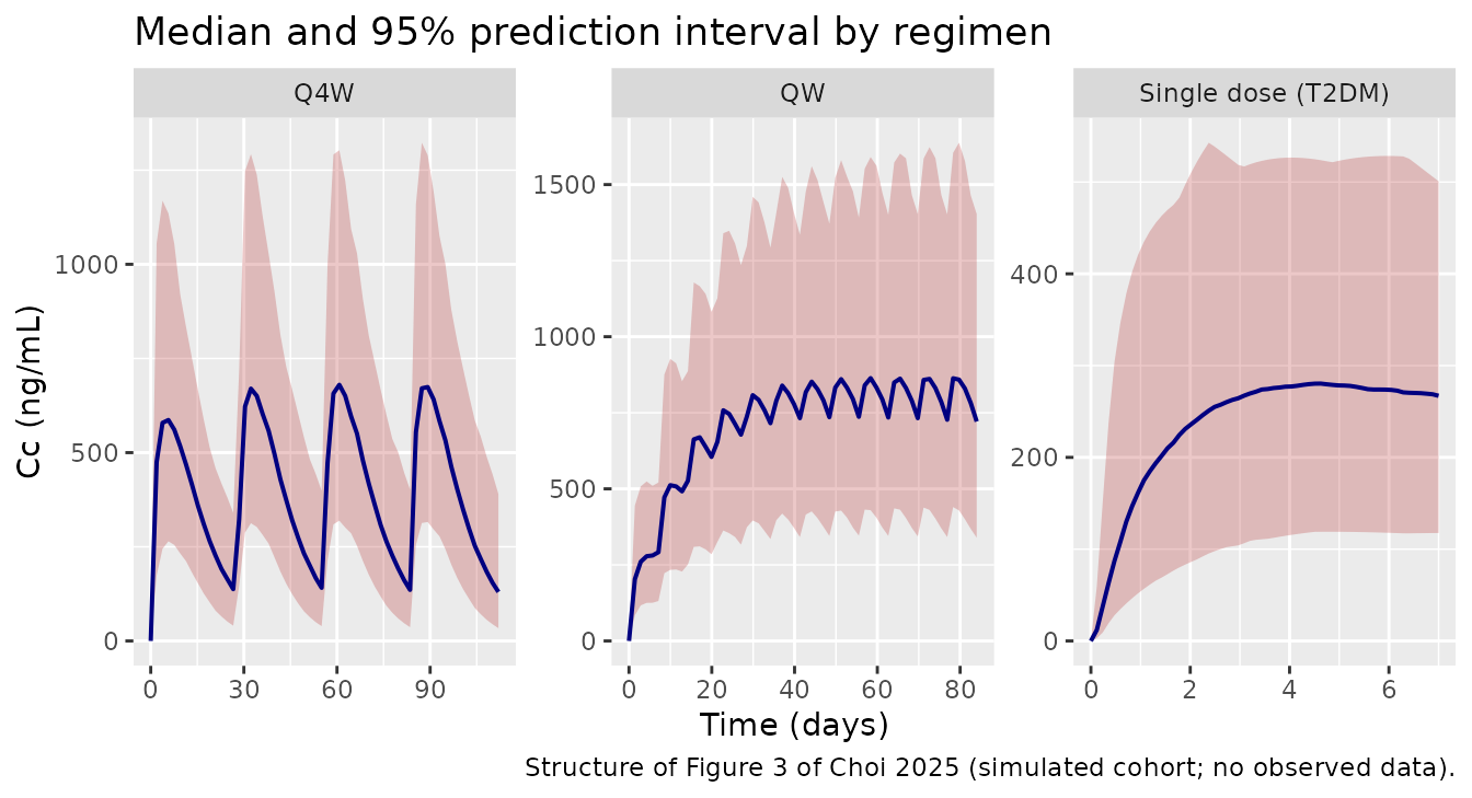
The width of that band is what settles the reading of the
residual-error estimate. Choi 2025 Table 3 reports
eps prop = 0.15 without stating whether 0.15 is the
proportional SD or the NONMEM $SIGMA variance. Read as a
variance the SD would be 0.387, whose residual contribution alone puts
the 2.5th percentile at 1 - 1.96 * 0.387 = 0.24 of the
prediction – already far below the lower edge of the paper’s own pcVPC
(Figure 3 panel C reads a lower-edge-to-median ratio of about 0.53)
before any IIV is added. The packaged model therefore takes
0.15 as the SD, and the check below confirms the resulting band is
compatible with Figure 3 rather than far wider than it.
band <- sim_vpc |>
  dplyr::filter(!is.na(Cc), regimen == "QW", time > 6 * tau) |>
  dplyr::group_by(time) |>
  dplyr::summarise(lo = quantile(Cc, 0.025), mid = median(Cc), .groups = "drop") |>
  dplyr::mutate(ratio = lo / mid)

cat(sprintf("lower-95%%-PI / median over the QW plateau: %.3f (Figure 3 reads ~0.5)\n",
            median(band$ratio)))
#> lower-95%-PI / median over the QW plateau: 0.486 (Figure 3 reads ~0.5)
# A variance reading of sigma would drive this ratio towards ~0.2; the SD
# reading keeps it near the ~0.5 the paper's pcVPC shows. The bound is wide
# enough to be cohort-independent but still separates the two readings, which
# differ by more than a factor of two.
stopifnot(median(band$ratio) > 0.33)
Assumptions and deviations / Errata
Structural encoding
-
The transit input rate carries the leading
Ktrthat Equation 4 drops. As printed, Equation 4’s second term isDose * BIOA2 * (Ktr*t)^n * exp(-Ktr*t) / n!, which has units of amount, not amount per time, and integrates toDose * BIOA2 / Ktrinstead ofDose * BIOA2. The paper’s own Equations 1-2 give the correct form: Equation 1 makes the outflow from the last transit compartmentKtr * a_nand Equation 2 givesa_n(t), so the depot input rate isKtr * a_n(t) = Dose * BIOA2 * Ktr * (Ktr*t)^n * exp(-Ktr*t) / n!– the Savic 2007 form, and exactly whatrxode2::transit()computes. Encoding Equation 4 literally would scale the transit arm by1/Ktr = 0.41. The mass-balance check above gates this. -
Exact gamma instead of Stirling’s approximation.
Equation 3 evaluates
n!for non-integernwithsqrt(2*pi) * n^(n+0.5) * exp(-n). rxode2 useslgamma(n+1). Atn = 5.52Stirling giveslog(n!) = 5.6834against the exact 5.6985, so the paper’s kernel amplitude is 1.5% high and its transit arm delivers 0.763 rather than 0.752 of the dose. The exact form is used here because it conserves mass exactly; 1.5% is an order of magnitude below the residual error. Same choice asLee_2015_sumatriptan. -
One depot, one
ka. Both absorption arms discharge into the same depot and shareka, per the Discussion (“both pathways were described using the same first-order rate constant (ka = 0.006 h-1)”). This differs from the siblingLee_2015_sumatriptandual-pathway model, which uses two depots with two distinct rate constants. -
Dose-record convention. Supply one
dose record targeting
depotwith the full administered amount.f(depot) <- ffoadmits the bolus fraction andtransit(nn, mtt, 1 - ffo)supplies the delayed fraction from the same (unscaled) record amount. -
IIV on
BIOA1is additive on the logit scale. Equation 7’s stated purpose is “to confine the estimated fraction values to the range between 0 and 1 and to allow implementation of interindividual variability”, so the eta sits onBIOF, not onBIOA1itself. Table 3’s 66.93% CV is converted with the paper’s own Equation 9 and applied on the logit scale. -
Diagonal OMEGA, no IOV. Results 3.1 reports “no
statistically significant covariance identified between IIV terms” and
that IOV “was evaluated but not found to be significant and was
therefore not included in the final model”. No IIV was reported on
Q/ForN, so those etas are absent rather than set to a guessed value.
Errata and internal inconsistencies in Choi 2025
-
Table 3 definition cell for the weight-on-CL/F
exponent. The row “Covariate effect (theta) of body weight on
CL/F” prints the definition
(V_C/F) x (WT/92)^theta, copied from thekarow’s template. The row label, Results 3.1 (“body weight influenced both ka and CL/F … exponents of -0.927 and 0.964, respectively”) and the Discussion (“a significant covariate on both ka and CL/F … normalized to 92 kg; the exponents of -0.927 and 0.964”) all place 0.964 on CL/F. Three statements against one cell; the model puts it on CL/F. The twelve-row Figure 6 reproduction above confirms this independently – a weight exponent on Vc would leave steady-state AUC weight-independent and flatten every row to 1.0. - Results 3.2 swaps the two weight-subgroup GMR labels. The text states that “the 10th percentile individual (79 kg) exhibited approximately 18% lower AUC and Cmax (GMR 0.82; 90% CI: 0.81-0.83), whereas the 90th percentile individual (120 kg) demonstrated about 20% higher exposure (GMR 1.22; 90% CI: 1.20-1.24)”. Figure 6 shows the opposite assignment – 79 kg at about 1.22 and the 90th-percentile weight at about 0.82 – and the Discussion agrees with the figure (“For a change from 96 to 79 kg (~17.7% decrease), AUC increased by approximately 20.7% and CL/F decreased by approximately 17.1%”). A positive exponent on CL/F necessarily makes the lighter subject the higher-exposure one. Figure 6 and the Discussion are correct; the Results sentence has the two labels transposed. The model reproduces the Discussion’s numbers exactly (20.67% AUC increase, 17.13% CL/F decrease for 96 -> 79 kg) and every Figure 6 row to within 1.1%.
- Figure 6 weight label: 119 vs 120 kg. The caption gives the 90th-percentile weight as 119 kg while Results 3.2 says 120 kg. 119 kg is used here because it is the caption’s simulation input and reproduces the printed 90% CI more closely.
- Obesity-vs-T2DM exposure ratio. Results 3.2 states that obese participants had “approximately 21% higher steady-state AUC compared to subjects with T2DM”, but Table 3’s two CL/F values imply 37.5% at a common body weight (the “38% higher clearance in T2DM” of the Discussion) and about 31% at the subgroup median weights. Figure 4B’s own plotted curves read roughly 1.24. Closing the gap to 1.21 would require the T2DM simulation to have used a body weight near 85 kg, below every per-study T2DM median in Table 2 (88-97.3 kg). The packaged model follows Table 3, which the Discussion’s effect-size statement confirms exactly; the 21% summary is not reproduced and is deliberately excluded from the assertion gate rather than accommodated by a widened tolerance.
-
Residual-error scale. Table 3 reports
eps prop = 0.15without stating whether this is the proportional SD or the$SIGMAvariance. It is taken as the SD; the pcVPC band argument is given in the section above. Were it a variance, the proportional SD would be 38.7%. -
MTTIIV precision. Table 3 gives the RSE of the MTT IIV as 37.14% while Results 3.1 gives 35.88% for the same term. This affects only the reported precision, not the 46.27% CV point estimate that the model uses. -
Table 2 internal arithmetic. Two inconsistencies
are reproduced as printed in the
populationmetadata rather than silently corrected: the Total age range (18-64 years) is narrower than the HM-EXC-201 per-study range (47-75 years), and the race counts sum to 501 rather than 498 (the “Others” row prints 13 subjects at 1.92%, but 13/498 = 2.61%). -
Specimen wording. Methods 2.2 states that “Serum
concentrations of efpeglenatide were quantified using a validated
ELISA”, while the same section, Section 2.7 and the axis labels of
Figures 2-5 all say plasma.
compartmentDatarecords plasma as the dominant designation.
Simulation assumptions in this vignette
- Original observed concentrations are not publicly available, so no panel here overlays real data; the Figure 3 replication shows model-predicted intervals only.
- Figure 4A of Choi 2025 does not state which population it was
simulated in. Its absolute concentrations are consistent with the T2DM
clearance (0.044 L/h) rather than the obesity clearance, so
DIS_DIAB = 1at 92 kg is used for that panel. The dose-proportionality and time-to-steady-state checks are unaffected by the choice. - Figure 4B’s per-population body weights are not given. The obese median (96 kg, from the Figure 6 caption) and the pooled T2DM median (92 kg, the model’s reference weight) are used; the resulting ratio is reported rather than gated.
- Ten of the twelve Figure 6 AUC ratios were digitised from the plotted symbols and carry about +/- 0.01 reading uncertainty; the 79 kg and 90th-percentile rows are printed numerically in Results 3.2 with 90% CIs. No parameter was adjusted to improve agreement.
- The screened-but-not-retained covariates (age, sex, race, BMI, lean
body mass) are recorded in the model file’s
covariatesDataExcludedlist. The paper’s five-level race screen is mapped onto the four registeredRACE_*canonicals; its “Native Hawaiian or Pacific Islander” level (2 participants) is folded intoRACE_OTHERbecause no canonical exists for it and the whole race covariate was rejected by the stepwise search.