Mycophenolic acid (Wei 2022) • nlmixr2lib

Model and source

Citation: Wei Y, Wu D, Chen Y, Dong C, Qi J, Wu Y, Cai R, Zhou S, Li C, Niu L, Wu T, Xiao Y, Liu T. Population pharmacokinetics of mycophenolate mofetil in pediatric patients early after liver transplantation. Front Pharmacol. 2022;13:1002628. doi:10.3389/fphar.2022.1002628.
Description: Two-compartment population PK model with first-order absorption and first-order elimination for mycophenolic acid (MPA) after oral mycophenolate mofetil dispersible tablets (MMFdt) in Chinese pediatric patients early after liver transplantation (Wei 2022). Body weight enters every structural parameter except Vp/F by fixed allometric scaling to a 7.5 kg reference (exponent 0.75 on CL/F and Q/F, 1 on Vc/F, -0.25 on Ka); the per-administration MMF dose in mg/kg enters CL/F as a power term normalised to 11.16 mg/kg. Vp/F is fixed at 269 L. Log-normal inter-individual variability on CL/F and Q/F only; exponential residual error.
Article: https://doi.org/10.3389/fphar.2022.1002628 (open access)

Wei 2022 reports no supplementary data files; the supplementary archive on Europe PMC holds only the six article figures. No correction notice was found on Europe PMC or the publisher page as of 2026-10-10.

Population

Wei 2022 enrolled 20 Chinese children (12 boys, 8 girls) receiving a first liver transplant at the First Affiliated Hospital of Guangxi Medical University in Nanning in 2020-2021 (Table 1). Median age was 0.74 years (IQR 0.61-1.69, range 0.42-7.76); 15 of the 20 were younger than 24 months. Median body weight was 7.5 kg (IQR 6.0-10.0, range 4.6-27.0). The main indication was liver cirrhosis after a Kasai operation (16 of 20). All children received mycophenolate mofetil dispersible tablets (MMFdt) orally or by nasogastric tube every 12 hours, together with tacrolimus and methylprednisolone. Doses started at 10-15 mg/kg and were adjusted clinically. On the sampling day the median dose was 11.2 mg/kg per dose (IQR 10.0-15.0, range 8.9-61.5). Samples were drawn at steady state, on post-operative day 12 (median; range 4-39), before and 0.5, 1, 2, 4, 8 and 12 h after the morning dose. After 7 samples below the detection limit were removed, 115 plasma MPA concentrations remained; the 21 below the 0.3 mg/L LLOQ were imputed as 0.15 mg/L (M5 method).

str(rxode2::rxode(readModelDb("Wei_2022_mycophenolic_acid"))$population, max.level = 1)
#> ℹ parameter labels from comments will be replaced by 'label()'
#> List of 17
#>  $ species       : chr "human"
#>  $ n_subjects    : int 20
#>  $ n_studies     : int 1
#>  $ n_observations: chr "115 MPA plasma concentrations (122 samples, 7 below the detection limit removed; the 21 remaining values below "| __truncated__
#>  $ age_range     : chr "0.42-7.76 years"
#>  $ age_median    : chr "0.74 years (IQR 0.61-1.69); 15 of 20 younger than 24 months"
#>  $ weight_range  : chr "4.6-27.0 kg"
#>  $ weight_median : chr "7.5 kg (IQR 6.0-10.0)"
#>  $ height_median : chr "67.5 cm (IQR 62.2-80.0)"
#>  $ bsa_median    : chr "0.39 m^2 (IQR 0.32-0.43)"
#>  $ sex_female_pct: num 40
#>  $ race_ethnicity: chr "Chinese (single centre, Nanning, Guangxi)."
#>  $ disease_state : chr "Pediatric first liver transplant recipients (16 liver cirrhosis after Kasai operation, 1 each biliary atresia, "| __truncated__
#>  $ dose_range    : chr "Oral or nasogastric MMF dispersible tablets q12h, starting 10-15 mg/kg per dose and adjusted clinically; 11.2 m"| __truncated__
#>  $ regions       : chr "China"
#>  $ co_medication : chr "Tacrolimus and methylprednisolone in all patients (triple regimen). Meropenem 55 %, voriconazole 50 %, furosemi"| __truncated__
#>  $ notes         : chr "Steady-state sampling from day 4 of MMFdt before and 0.5, 1, 2, 4, 8 and 12 h after the morning dose (Wei 2022 "| __truncated__

Source trace

The PDF’s final-model equations (Results, Equations 1-5) are the primary source; the abstract restates them. Table 3 gives the same estimates rounded.

Equation / parameter	Value	Source location
`lcl` (CL/F at 7.5 kg, 11.16 mg/kg)	log(14.8) L/h	Equation 1; Table 3
`lka` (Ka at 7.5 kg)	log(2.02) 1/h	Equation 2 (Table 3 rounds to 2.0)
`lvc` (Vc/F at 7.5 kg)	log(6.01) L	Equation 3 (Table 3 rounds to 6.0)
`lvp` (Vp/F)	fixed(log(269)) L	Equation 4 (“fixed”); Table 3
`lq` (Q/F at 7.5 kg)	log(15.4) L/h	Equation 5; Table 3
`e_wt_cl`, `e_wt_q`	fixed 0.75	Equations 1 and 5
`e_wt_vc`	fixed 1	Equation 3
`e_wt_ka`	fixed -0.25	Equation 2
`e_dose_cl`	0.452	Equation 1; Table 3 theta_DOSE
Dose normaliser	11.16 mg/kg	Equation 1
`etalcl`	variance 0.06	Equation 1 term `e^0.06` (printed as `f ^ 0.06`); Table 3 IIV CL/F 24.5 % = sqrt(0.06)
`etalq`	variance 1.39	Equation 5 term `e^1.39`; Table 3 IIV Q/F 117.9 % = sqrt(1.39)
`expSd`	0.503	Table 3 RV 50.3 %; Results: “IIV and RV were represented as exponents”
Structure	2-cmt, first-order absorption and elimination	Abstract; Results “Population pharmacokinetic model”

Virtual cohort

Two arms of 200 virtual children each, dosed every 12 hours for 10 days (20 doses, steady state), with dense sampling over the final interval.

Reference: every child at the 7.5 kg / 11.16 mg/kg reference. Figure 4 of Wei 2022 is a prediction-corrected VPC, which normalises each observation to the typical prediction at its covariates, so a reference-covariate cohort is the comparable simulation.
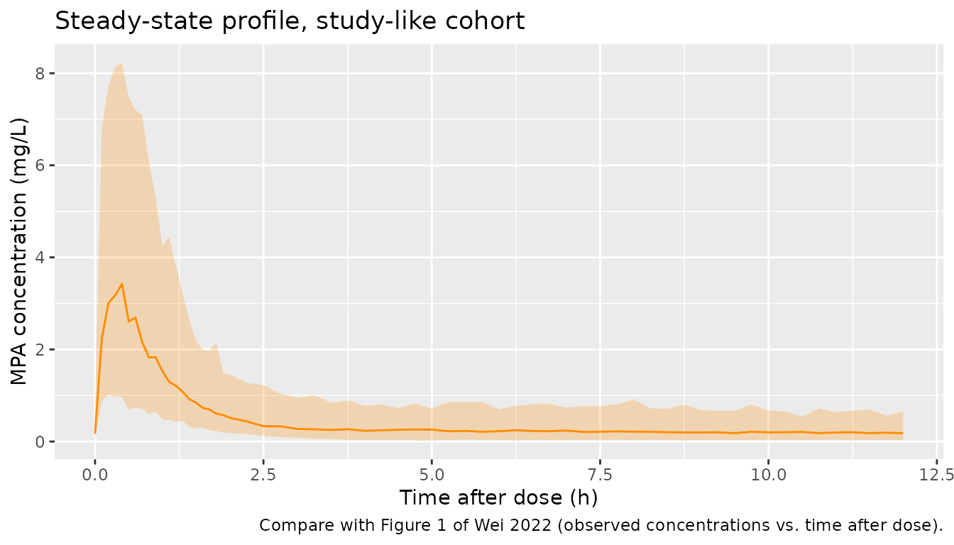
Study-like: weight and dose per kg drawn to match Table 1. Weight is log-normal with median 7.5 kg and log-SD 0.379, from IQR 6.0-10.0, truncated to 4.6-27 kg. Dose per kg is log-normal with median 11.16 mg/kg and log-SD 0.30, from IQR 10-15, truncated to 8.9-61.5 mg/kg.

set.seed(20221013)

n_per_arm <- 200L
dose_times <- seq(0, 228, by = 12)
obs_times <- c(seq(228, 230, by = 0.1), seq(230.25, 240, by = 0.25))

rtrunc_lnorm <- function(n, median, sdlog, lo, hi) {
  x <- rlnorm(n, log(median), sdlog)
  bad <- x < lo | x > hi
  while (any(bad)) {
    x[bad] <- rlnorm(sum(bad), log(median), sdlog)
    bad <- x < lo | x > hi
  }
  x
}

make_cohort <- function(subjects, arm) {
  doses <- tidyr::crossing(subjects, time = dose_times) |>
    mutate(evid = 1L, cmt = "depot", amt = DOSE_MMF_MGKG * WT)
  obs <- tidyr::crossing(subjects, time = obs_times) |>
    mutate(evid = 0L, cmt = "central", amt = 0)
  bind_rows(doses, obs) |>
    mutate(arm = arm) |>
    select(id, time, evid, amt, cmt, WT, DOSE_MMF_MGKG, arm) |>
    arrange(id, time, desc(evid))
}

ref_subj <- tibble(id = seq_len(n_per_arm), WT = 7.5, DOSE_MMF_MGKG = 11.16)
study_subj <- tibble(
  id = n_per_arm + seq_len(n_per_arm),
  WT = rtrunc_lnorm(n_per_arm, 7.5, 0.379, 4.6, 27),
  DOSE_MMF_MGKG = rtrunc_lnorm(n_per_arm, 11.16, 0.30, 8.9, 61.5)
)

events <- bind_rows(
  make_cohort(ref_subj, "Reference (7.5 kg, 11.16 mg/kg)"),
  make_cohort(study_subj, "Study-like (Table 1)")
)
stopifnot(!anyDuplicated(unique(events[, c("id", "time", "evid")])))

summary(study_subj[, c("WT", "DOSE_MMF_MGKG")])
#>        WT         DOSE_MMF_MGKG   
#>  Min.   : 4.727   Min.   : 8.919  
#>  1st Qu.: 6.624   1st Qu.:10.336  
#>  Median : 8.107   Median :11.575  
#>  Mean   : 8.442   Mean   :12.528  
#>  3rd Qu.: 9.406   3rd Qu.:13.595  
#>  Max.   :17.751   Max.   :31.240

Simulation

mod <- readModelDb("Wei_2022_mycophenolic_acid")
rxode2::rxSetSeed(20221013)
sim <- rxode2::rxSolve(mod, events = events, keep = c("arm", "WT", "DOSE_MMF_MGKG")) |>
  as.data.frame() |>
  mutate(tad = time - 228)
#> ℹ parameter labels from comments will be replaced by 'label()'

sim_typ <- rxode2::rxSolve(rxode2::zeroRe(mod), events = filter(events, id == 1L)) |>
  as.data.frame() |>
  mutate(tad = time - 228)
#> ℹ parameter labels from comments will be replaced by 'label()'
#> ℹ omega/sigma items treated as zero: 'etalcl', 'etalq'

Cc in the output is the individual prediction; sim adds the exponential residual error.

Replicate published figures

The points below are the median (solid red line) and 95th percentile (upper dashed red line) of Figure 4 of Wei 2022, a prediction-corrected VPC, read off the figure by the maintainers. The figure caption describes these lines as the simulated median and 90 % prediction interval, and the shaded bands as their 95 % confidence intervals. Either way they are the paper’s own summary of the steady-state profile at the reference covariates.

fig4_obs <- tibble::tribble(
  ~tad, ~Q50, ~Q95,
  0,    0.15, 0.7,
  0.5,  2.4,  11.8,
  1,    1.5,  5.2,
  2,    0.45, 1.6,
  4,    0.22, 0.65,
  8,    0.18, 0.85,
  12,   0.15, 0.62
)

vpc <- sim |>
  filter(arm == "Reference (7.5 kg, 11.16 mg/kg)") |>
  group_by(tad) |>
  summarise(
    Q05 = quantile(sim, 0.05),
    Q50 = quantile(sim, 0.50),
    Q95 = quantile(sim, 0.95),
    .groups = "drop"
  )

ggplot(vpc, aes(tad)) +
  geom_ribbon(aes(ymin = Q05, ymax = Q95), fill = "steelblue", alpha = 0.25) +
  geom_line(aes(y = Q50), colour = "steelblue") +
  geom_point(data = fig4_obs, aes(y = Q50), colour = "red") +
  geom_point(data = fig4_obs, aes(y = Q95), colour = "red", shape = 2) +
  labs(
    x = "Time after dose (h)", y = "MPA concentration (mg/L)",
    title = "Steady-state VPC at the reference covariates",
    caption = paste(
      "Replicates Figure 4 of Wei 2022. Band: simulated 5th-95th percentile;",
      "line: simulated median; red: Figure 4 median (circles) and 95th percentile (triangles)."
    )
  )

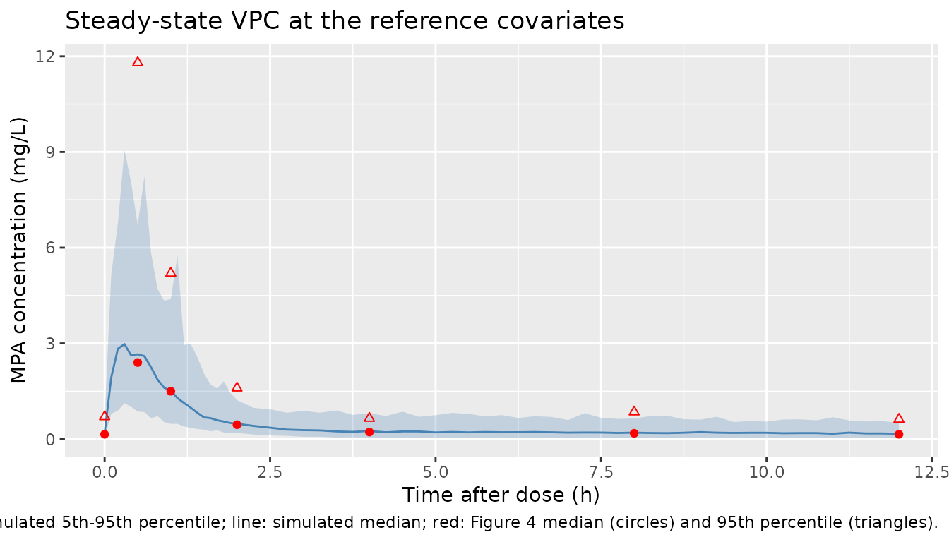
fig4_cmp <- fig4_obs |>
  left_join(
    vpc |> rename(sim_Q50 = Q50, sim_Q95 = Q95) |> mutate(tad = round(tad, 2)),
    by = "tad"
  ) |>
  select(tad, Q50, sim_Q50, Q95, sim_Q95)
fig4_cmp |>
  rename(
    "Time after dose (h)" = tad,
    "Figure 4 median" = Q50,
    "Simulated median" = sim_Q50,
    "Figure 4 95th" = Q95,
    "Simulated 95th" = sim_Q95
  ) |>
  knitr::kable(digits = 2, caption = "Figure 4 percentiles vs. this simulation (mg/L).")

Figure 4 percentiles vs. this simulation (mg/L).
Time after dose (h)	Figure 4 median	Simulated median	Figure 4 95th	Simulated 95th
0.0	0.15	0.17	0.70	0.60
0.5	2.40	2.66	11.80	6.70
1.0	1.50	1.52	5.20	4.39
2.0	0.45	0.48	1.60	1.22
4.0	0.22	0.25	0.65	0.81
8.0	0.18	0.20	0.85	0.65
12.0	0.15	0.16	0.62	0.51


# The typical-value peak and trough set the location of the whole profile; a
# wrong CL/F, Vc/F or dose unit moves them several-fold. The bounds are the
# 95 % CI band of the simulated median drawn in Figure 4 (about 1.4-3.7 mg/L
# at 0.5 h, about 0.1-0.4 mg/L from 4 h on).
typ_peak <- sim_typ$Cc[which.min(abs(sim_typ$tad - 0.5))]
typ_trough <- sim_typ$Cc[which.min(abs(sim_typ$tad - 12))]
stopifnot(
  typ_peak > 1.4, typ_peak < 3.7,
  typ_trough > 0.1, typ_trough < 0.4
)
c(typical_peak_0.5h = typ_peak, typical_trough_12h = typ_trough)
#>  typical_peak_0.5h typical_trough_12h 
#>          2.8762833          0.2072095

Compare the simulated median and 95th percentile with the Figure 4 values in the table above. Figure 4 summarises only 20 children, so its upper percentile is noisy.

The study-like cohort shows the spread that weight and dose add to the reference-covariate profile, for comparison with the raw observations in Figure 1 of Wei 2022 (peaks up to about 10 mg/L, troughs mostly 0.15-1.3 mg/L).

sim |>
  filter(arm == "Study-like (Table 1)") |>
  group_by(tad) |>
  summarise(
    Q05 = quantile(sim, 0.05),
    Q50 = quantile(sim, 0.50),
    Q95 = quantile(sim, 0.95),
    .groups = "drop"
  ) |>
  ggplot(aes(tad)) +
  geom_ribbon(aes(ymin = Q05, ymax = Q95), fill = "darkorange", alpha = 0.25) +
  geom_line(aes(y = Q50), colour = "darkorange") +
  labs(
    x = "Time after dose (h)", y = "MPA concentration (mg/L)",
    title = "Steady-state profile, study-like cohort",
    caption = "Compare with Figure 1 of Wei 2022 (observed concentrations vs. time after dose)."
  )

PKNCA validation

Wei 2022 reports no NCA parameters. The steady-state check instead uses mass balance: over a dosing interval at steady state the area under the curve equals the dose divided by the individual apparent clearance, AUCtau = Dose / CL/F. PKNCA computes AUCtau from the individual predictions (no residual error) and the comparison uses each child’s own clearance.

sim_nca <- sim |>
  filter(!is.na(Cc)) |>
  select(id, time, Cc, arm)

conc_obj <- PKNCA::PKNCAconc(sim_nca, Cc ~ time | arm + id)
dose_df <- events |>
  filter(evid == 1L) |>
  select(id, time, amt, arm)
dose_obj <- PKNCA::PKNCAdose(dose_df, amt ~ time | arm + id)

intervals <- data.frame(
  start = 228, end = 240,
  cmax = TRUE, tmax = TRUE, cmin = TRUE, auclast = TRUE
)
nca_res <- PKNCA::pk.nca(PKNCA::PKNCAdata(conc_obj, dose_obj, intervals = intervals))

nca_wide <- as.data.frame(nca_res$result) |>
  select(arm, id, PPTESTCD, PPORRES) |>
  tidyr::pivot_wider(names_from = PPTESTCD, values_from = PPORRES)

nca_wide |>
  group_by(arm) |>
  summarise(
    cmax = median(cmax), tmax = median(tmax), cmin = median(cmin),
    auclast = median(auclast), .groups = "drop"
  ) |>
  rename(
    "Arm" = arm,
    "Cmax (mg/L)" = cmax,
    "Tmax (h)" = tmax,
    "Cmin (mg/L)" = cmin,
    "AUC0-12 (mg*h/L)" = auclast
  ) |>
  knitr::kable(digits = 2, caption = "Median steady-state NCA by arm (individual predictions).")

Median steady-state NCA by arm (individual predictions).
Arm	Cmax (mg/L)	Tmax (h)	Cmin (mg/L)	AUC0-12 (mg*h/L)
Reference (7.5 kg, 11.16 mg/kg)	3.25	0.3	0.18	5.51
Study-like (Table 1)	3.41	0.3	0.20	5.79

cl_ind <- sim |>
  filter(time == 228) |>
  distinct(id, cl)
mb <- nca_wide |>
  left_join(cl_ind, by = "id") |>
  left_join(distinct(dose_df, id, amt), by = "id") |>
  mutate(
    auc_expected = amt / cl,
    pct_diff = 100 * (auclast - auc_expected) / auc_expected
  )

# Both sides use the same drawn parameters, so the difference is linear-
# trapezoidal error on the 0.1-h peak grid plus any residual approach to steady
# state. A wrong clearance or dose unit moves the median by far more than 5 %.
stopifnot(
  abs(median(mb$pct_diff)) < 5,
  quantile(abs(mb$pct_diff), 0.9) < 10
)
summary(mb$pct_diff)
#>     Min.  1st Qu.   Median     Mean  3rd Qu.     Max. 
#> -4.51876 -1.08663 -0.58024 -0.94621 -0.45327 -0.06027

At the reference covariates the typical AUCtau is 83.7 mg / 14.8 L/h = 5.7 mgh/L. That is well below the 30-60 mgh/L MPA target window quoted in the Wei 2022 Introduction, because the paper’s apparent clearance of 14.8 L/h in a 7.5 kg child is high. The model reproduces the low concentrations Wei 2022 observed (Figures 1 and 4); it does not reach the adult target range.

Assumptions and deviations

Dose covariate units. Wei 2022 defines DOSE only as “the MMFdt administered dose”. The maintainers read it as mg/kg per administration because the normaliser 11.16 matches the Table 1 median of 11.2 mg/kg per dose. A total dose in mg would be about 84 mg for a 7.5 kg child. The covariate is named DOSE_MMF_MGKG; set it to amt / WT on each dose.
Dose mass scale. Doses are entered as MMF mg. The paper reports no MPA-equivalent conversion, so the apparent CL/F, Vc/F, Q/F and Vp/F are taken to absorb the MMF-to-MPA mass ratio (0.739) along with bioavailability. The typical-value profile matches the Figure 4 median on this basis (0.5 h simulated about 2.9 mg/L vs. 2.4 mg/L in the figure). With MPA-equivalent dosing it would be about 2.1 mg/L, so the figure cannot cleanly separate the two readings.
IIV variances. The equations print the random effects as f ^ 0.06 and f ^ 1.39, a rendering of e^eta with the variance as the exponent. The maintainers used 0.06 and 1.39 directly as the log-scale variances. Table 3’s 24.5 % and 117.9 % are their square roots.
Residual error. “Exponential” residual error with RV 50.3 % is encoded as lnorm(expSd) with expSd = 0.503.
Ka and Vc/F precision. The equations print 2.02 h^-1 and 6.01 L; Table 3 rounds these to 2.0 and 6.0. The equation values are used.
Screened but not retained covariates. ALT and GRWR on CL/F, and UGT1A8 518C>G and SLCO1B1 521T>C on Q/F, entered during forward selection (Table 2) and were removed. They are documented in covariatesDataExcluded.
Virtual cohort. Weight and dose-per-kg distributions are log-normal fits to the Table 1 medians and IQRs, independent of each other. The 10-day dosing history stands in for each child’s actual post-transplant history.
Figure 4 values. The median and 95th-percentile lines were read off the published figure by the maintainers to about +/- 0.1 mg/L.