Model and source
- Citation: Ashraf MW, Poikola S, Neuvonen M, Kiiski JI, Kontinen VK, Olkkola KT, Backman JT, Niemi M, Saari TI. Population Pharmacokinetic Quantification of CYP2D6 Activity in Codeine Metabolism in Ambulatory Surgical Patients for Model-Informed Precision Dosing. Clin Pharmacokinet. 2024;63(11):1547-1560. doi:10.1007/s40262-024-01433-9.
- Description: Joint parent + three-metabolite population PK model for oral codeine and its metabolites morphine, codeine-6-glucuronide (C6G) and morphine-3-glucuronide (M3G) in 997 ambulatory surgical patients given a single preoperative 60 mg oral codeine dose (Ashraf 2024). Codeine is described by a one-compartment disposition with a first-order absorption depot and an estimated bioavailability. Total codeine elimination is split into a CYP2D6-mediated branch (ke * fm_morphine) that forms morphine and a non-CYP2D6 (glucuronidation) branch (ke * (1 - fm_morphine)) that forms C6G; morphine elimination is in turn split into an M3G-forming branch (ke_morphine * fm_m3g, fm_m3g fixed at 0.60 from the literature) and other pathways. Morphine, C6G and M3G each have a one-compartment disposition. The CYP2D6 activity score (CPIC sum of allele activity values) enters as an ordinal continuous covariate on the codeine-to-morphine metabolic fraction through an exponential model referenced to an activity score of 2, followed by the authors’ f / (1 + f) rescaling that constrains the fraction to (0, 1). Codeine and morphine clearance and central volume are allometrically scaled to the population median body weight of 80 kg with fixed exponents 0.75 and 1; the glucuronide parameters are not weight-scaled.
- Article: https://doi.org/10.1007/s40262-024-01433-9 (open access, CC BY-NC)
- Online Resource 1 (methods, equations, supplementary figures): https://static-content.springer.com/esm/art%3A10.1007%2Fs40262-024-01433-9/MediaObjects/40262_2024_1433_MOESM1_ESM.pdf
- Online Resource 2 (CYP2D6 genotype distribution): https://static-content.springer.com/esm/art%3A10.1007%2Fs40262-024-01433-9/MediaObjects/40262_2024_1433_MOESM2_ESM.pdf
Codeine is a prodrug. CYP2D6 O-demethylates it to morphine, the species that carries essentially all of the analgesic (and respiratory-depressant) activity, while the much larger non-CYP2D6 branch glucuronidates it to the inactive codeine-6-glucuronide (C6G). Morphine is in turn largely glucuronidated to morphine-3-glucuronide (M3G). Because CYP2D6 is highly polymorphic, the fraction of a codeine dose that becomes morphine varies enormously between patients, and that variation is the clinical risk: poor metabolisers get little analgesia, ultrarapid metabolisers can reach morphine concentrations associated with respiratory depression.
Ashraf 2024 quantified that relationship prospectively in 997 ambulatory surgical patients, using the CPIC activity score (AS) as an ordinal continuous covariate rather than the conventional four-level metaboliser phenotype.
Population
The model was built on a single prospective trial (EudraCT 2015-005561-23) run at the Jorvi Hospital day-surgery unit in Espoo, Finland between August 2016 and March 2018. Of 1000 recruited patients, 997 contributed concentration data for at least one analyte. Every patient received a single preoperative oral paracetamol 1000 mg + codeine 60 mg combination tablet; use of strong CYP2D6 inhibitors was an exclusion criterion.
Baseline characteristics (paper Table 1) were mean (SD) age 47.8 (12.9) years, weight 79.8 (13.8) kg and BMI 25.9 (3.60) kg/m^2, with ASA physical status class 1 in 513 (51%), class 2 in 424 (43%) and class 3 in 60 (6%) patients. Sampling was deliberately sparse: exactly two blood samples per patient, the first 20-60 min and the second 180-360 min after the tablet. Codeine, morphine, C6G and M3G were assayed by LC-MS/MS with a 0.05 ng/mL lower limit of quantification and day-to-day CV below 11%.
All 997 patients were genotyped for the CYP2D6 variants defining the *1, *2, *3, *4, *5, *6, *9, *10, *15, *17, *35, *39 and *41 alleles plus copy-number variation; 64 distinct genotypes were observed. The resulting activity-score distribution (paper Table 1) is the covariate distribution used for the virtual cohorts below.
pop <- rxode2::rxode(readModelDb("Ashraf_2024_codeine"))$population
str(pop, max.level = 1)
#> List of 14
#>  $ species       : chr "human"
#>  $ n_subjects    : num 997
#>  $ n_studies     : num 1
#>  $ age_mean_sd   : chr "47.8 (12.9) years"
#>  $ weight_mean_sd: chr "79.8 (13.8) kg"
#>  $ weight_median : chr "80 kg (allometric reference)"
#>  $ bmi_mean_sd   : chr "25.9 (3.60) kg/m^2"
#>  $ sex_female_pct: NULL
#>  $ race_ethnicity: NULL
#>  $ disease_state : chr "Adults scheduled for elective ambulatory (day-case) surgery. American Society of Anesthesiologists physical sta"| __truncated__
#>  $ dose_range    : chr "Single preoperative oral dose of codeine 60 mg given as a paracetamol 1000 mg + codeine 60 mg combination table"| __truncated__
#>  $ regions       : chr "Finland (Jorvi Hospital day-surgery unit, Espoo)"
#>  $ genotype      : chr "CYP2D6 activity score distribution (n, % of 997): AS 0, 37 (3.7); 0.25, 5 (0.5); 0.5, 21 (2.1); 0.75, 2 (0.2); "| __truncated__
#>  $ notes         : chr "Demographics from paper Table 1. Prospective clinical trial (EudraCT 2015-005561-23), 1000 patients recruited, "| __truncated__
Source trace
Every ini() entry in
inst/modeldb/specificDrugs/Ashraf_2024_codeine.R carries an
in-file comment naming its source location. They are collected here for
review.
| Equation / parameter | Value | Source location |
|---|---|---|
lka |
8.74 1/h | Table 2, k_a,cod
|
lcl |
110 L/h | Table 2, CL_cod
|
lvc |
427.5 L | Table 2, V_c,cod
|
lfdepot |
0.84 | Table 2, F_cod
|
lcl_morphine |
357.5 L/h | Table 2, CL_mor
|
lvc_morphine |
22.8 L | Table 2, V_c,mor
|
lcl_c6g |
7.96 L/h | Table 2, CL_C6G
|
lvc_c6g |
5.36 L | Table 2, V_c,C6G
|
lcl_m3g |
9.45 L/h | Table 2, CL_M3G
|
lvc_m3g |
8.47 L | Table 2, V_c,M3G
|
lfm_morphine |
0.16 | Table 2, f_mor (footnote b: “Scaled to activity score
2”) |
lfm_m3g |
0.60 (fixed) | Section 3.1 and Online Resource 1 Section 2.1 (“fixed at 60%, according to a recent report”) |
e_cyp2d6_fm_morphine |
1.00 | Table 2, GEN_eff
|
e_wt_cl_q |
0.75 (fixed) | Online Resource 1 Eq. 3 |
e_wt_vc_vp |
1 (fixed) | Online Resource 1 Eq. 4 |
etalka |
3.75 | Table 2, eta k_a,cod
|
etalvc |
0.181 | Table 2, eta V_c,cod
|
etalfdepot |
0.024 | Table 2, eta F_cod
|
etalcl_morphine |
0.062 | Table 2, eta CL_mor
|
etalfm_morphine |
0.334 | Table 2, eta R_mor
|
expSd |
0.259 | Table 2, epsilon_cod
|
expSd_morphine |
0.149 | Table 2, epsilon_mor
|
expSd_c6g |
0.103 | Table 2, epsilon_C6G
|
expSd_m3g |
0.096 | Table 2, epsilon_M3G
|
| Compartment structure and branch fractions | n/a | Figure 1 schematic |
| Allometric scaling equations | n/a | Online Resource 1 Eqs. 3-6; paper Section 2.5 |
| CYP2D6 exponential covariate model | n/a | Online Resource 1 Eq. 11; paper Section 3.2 |
IIV applied before the f / (1 + f) rescaling |
n/a | Online Resource 1 Eqs. 13-14 |
| Activity-score assignment rules | n/a | Table 1 footnote a |
| Reference weight 80 kg | n/a | Online Resource 1 Eqs. 3-4; paper Section 2.6 |
| Reference activity score 2 | n/a | Paper Section 3.2; Table 2 footnote b |
The CYP2D6 activity-score covariate
The paper tested categorical (metaboliser-phenotype) and continuous (activity-score) parameterisations of the CYP2D6 effect on the codeine-to-morphine metabolic fraction, and retained the exponential activity-score form. Online Resource 1 Eqs. 11, 13 and 14 give the full chain:
with
,
and
.
The final f / (1 + f) step is what keeps the fraction
inside
:
without it the typical value at AS 4 would be
,
which is not a fraction.
as_grid <- seq(0, 4, by = 0.05)
fm_raw <- 0.16 * exp(1.00 * (as_grid - 2))
fm_curve <- tibble(
  AS = rep(as_grid, 2),
  fm = c(fm_raw, fm_raw / (1 + fm_raw)),
  form = rep(c("Before f/(1+f) rescaling", "Final model (Eq. 14)"), each = length(as_grid))
)

# Paper Figure 3B / Section 3.3: median apparent CYP2D6 activity, expressed as a
# percentage of total codeine clearance, in each metaboliser-phenotype class.
observed_median <- tibble(
  AS = c(0, 1, 2, 3),
  fm = c(0.0055, 0.0682, 0.138, 0.199),
  label = c("PM", "IM", "NM", "UM")
)

ggplot(fm_curve, aes(AS, 100 * fm, colour = form)) +
  geom_line(linewidth = 0.9) +
  geom_point(data = observed_median, aes(AS, 100 * fm), inherit.aes = FALSE,
             size = 3, shape = 21, fill = "white") +
  geom_text(data = observed_median, aes(AS, 100 * fm, label = label),
            inherit.aes = FALSE, vjust = -1, size = 3) +
  geom_hline(yintercept = 100, linetype = "dotted") +
  labs(x = "CYP2D6 activity score", y = "Fraction of codeine metabolised to morphine (%)",
       colour = NULL,
       title = "CYP2D6 activity score drives the codeine-to-morphine fraction",
       caption = paste("Points are the median apparent CYP2D6 activity per metaboliser class",
                       "reported in Ashraf 2024 Section 3.3 (Figure 3B),\nplotted at the modal",
                       "activity score of each class. Dotted line marks 100%.")) +
  theme(legend.position = "bottom")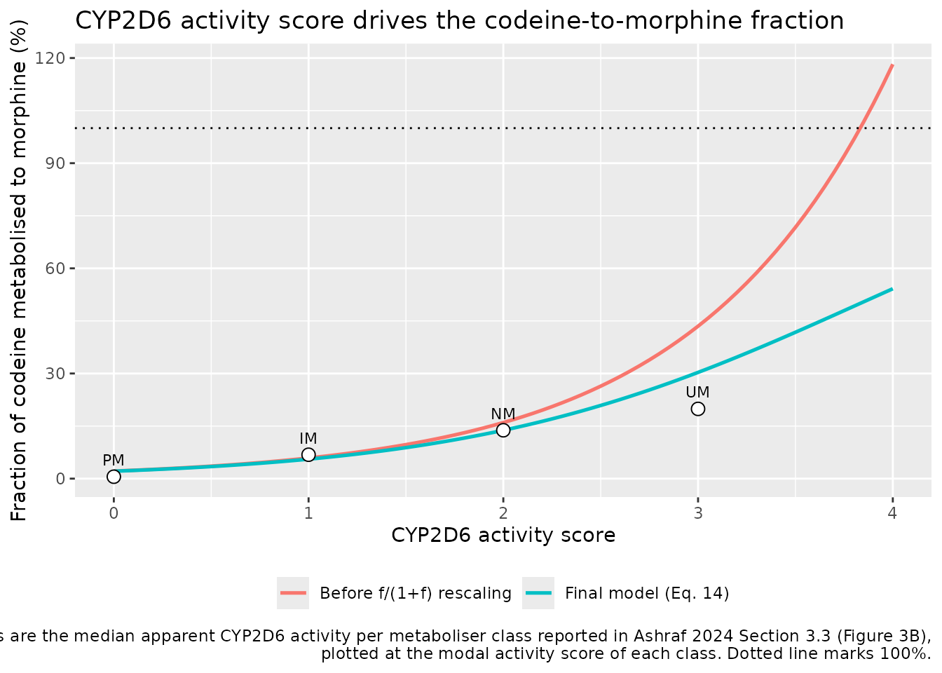
The typical value at AS 2 is 13.8%, which reproduces the paper’s
reported normal-metaboliser median apparent CYP2D6 activity of 13.8% of
total codeine clearance almost exactly. The uncorrected exponential
(upper curve) exceeds 100% above AS 3.7, confirming that the
f / (1 + f) step is part of the final model rather than an
intermediate step in model development.
Virtual cohort
Original patient-level data are not available (the paper states they cannot be shared because of re-identification risk). The cohorts below reproduce the published covariate distributions: body weight drawn from the reported mean (SD) of 79.8 (13.8) kg, and CYP2D6 activity score drawn from the exact Table 1 frequency distribution.
set.seed(20241023)

n_vpc <- 200  # subjects in the VPC cohort (200 per arm cap)

# Paper Table 1: CYP2D6 activity score distribution among the 997 patients.
as_levels <- c(0, 0.25, 0.5, 0.75, 1, 1.25, 1.5, 2, 2.25, 3, 4)
as_counts <- c(37, 5, 21, 2, 240, 23, 67, 537, 2, 61, 2)

draw_wt <- function(n) pmin(pmax(rnorm(n, 79.8, 13.8), 45), 140)

subj_vpc <- tibble(
  id = seq_len(n_vpc),
  WT = draw_wt(n_vpc),
  CYP2D6 = sample(as_levels, n_vpc, replace = TRUE, prob = as_counts / sum(as_counts))
)

obs_times <- sort(unique(c(seq(0, 1.5, by = 0.05), seq(1.5, 6, by = 0.1))))

make_events <- function(subj, dose_mg, times, dose_times = 0) {
  doses <- subj |>
    tidyr::crossing(time = dose_times) |>
    mutate(amt = dose_mg, evid = 1L, cmt = "depot", dvid = NA_integer_)
  obs <- subj |>
    tidyr::crossing(time = times) |>
    mutate(amt = NA_real_, evid = 0L, cmt = "central", dvid = 1L)
  bind_rows(doses, obs) |> arrange(id, time, desc(evid))
}

events_vpc <- make_events(subj_vpc, dose_mg = 60, times = obs_times)
stopifnot(!anyDuplicated(unique(events_vpc[, c("id", "time", "evid")])))
Simulation
mod <- readModelDb("Ashraf_2024_codeine")

# useLinCmt = FALSE: rxode2's automatic ODE -> linCmt conversion corrupts the
# dvid -> cmt mapping for multi-output models such as this one.
sim_vpc <- rxode2::rxSolve(
  mod, events = events_vpc,
  keep = c("WT", "CYP2D6"),
  useLinCmt = FALSE
) |>
  as.data.frame()
Replicate published figures
Figure 2 – visual predictive checks
Paper Figure 2 shows VPCs for all four analytes after a single 60 mg oral codeine dose over the first 6 h. Note that the published panel labels for morphine and C6G are transposed relative to the plotted data: the panel with concentrations of order 1-10 ng/mL is morphine and the panel of order 1000 ng/mL is C6G (C6G exposure exceeds morphine exposure roughly 350-fold in this model). The panels below are labelled by analyte.
# Replicates Figure 2 of Ashraf 2024: median and 5th-95th percentiles of the
# simulated plasma concentrations of each analyte after 60 mg oral codeine.
vpc_long <- sim_vpc |>
  filter(time > 0) |>
  transmute(
    id, time,
    Codeine = 1000 * Cc,
    Morphine = 1000 * Cc_morphine,
    `Codeine-6-glucuronide` = 1000 * Cc_c6g,
    `Morphine-3-glucuronide` = 1000 * Cc_m3g
  ) |>
  tidyr::pivot_longer(-c(id, time), names_to = "analyte", values_to = "conc") |>
  mutate(analyte = factor(analyte, levels = c(
    "Codeine", "Morphine", "Codeine-6-glucuronide", "Morphine-3-glucuronide")))

vpc_long |>
  group_by(analyte, time) |>
  summarise(
    Q05 = quantile(conc, 0.05), Q50 = median(conc), Q95 = quantile(conc, 0.95),
    .groups = "drop"
  ) |>
  ggplot(aes(time, Q50)) +
  geom_ribbon(aes(ymin = Q05, ymax = Q95), alpha = 0.25, fill = "steelblue") +
  geom_line(linewidth = 0.8) +
  facet_wrap(~analyte, scales = "free_y") +
  scale_y_log10() +
  labs(x = "Time after codeine dose (hours)", y = "Plasma concentration (ng/mL)",
       title = "Figure 2 -- simulated VPC after 60 mg oral codeine",
       caption = "Replicates Figure 2 of Ashraf 2024. Line = median, band = 5th-95th percentile.")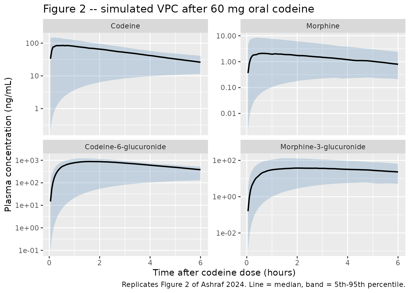
The observed medians read off paper Figure 2 at 1 h are approximately 65 ng/mL for codeine, 3-4 ng/mL for morphine, 1000-1500 ng/mL for C6G and 50-90 ng/mL for M3G. The simulated medians below are on the same scale for all four analytes. The codeine median sits below its typical-value prediction (93.9 ng/mL at 1 h) because of the very large IIV on the absorption rate constant, which pushes a substantial share of the population into a slow-absorption regime at 1 h.
vpc_long |>
  filter(time %in% c(0.5, 1, 2, 6)) |>
  group_by(analyte, time) |>
  summarise(`Simulated median (ng/mL)` = median(conc), .groups = "drop") |>
  tidyr::pivot_wider(names_from = time, values_from = `Simulated median (ng/mL)`,
                     names_prefix = "t = ") |>
  dplyr::rename(Analyte = analyte) |>
  knitr::kable(digits = 1,
caption = "Simulated median plasma concentrations (ng/mL) after 60 mg oral codeine.")| Analyte | t = 0.5 | t = 1 | t = 2 | t = 6 |
|---|---|---|---|---|
| Codeine | 84.3 | 80.1 | 65.5 | 26.0 |
| Morphine | 2.1 | 1.9 | 1.7 | 0.8 |
| Codeine-6-glucuronide | 517.1 | 775.9 | 869.8 | 384.1 |
| Morphine-3-glucuronide | 15.5 | 30.3 | 37.7 | 23.1 |
Figure 4 – typical-patient dosing scenarios
Paper Figure 4 simulates a typical patient given 60 mg codeine once, twice, three or four times daily and plots morphine concentrations against the previously reported 9.1 ng/mL EC50 for respiratory depression. That figure is a typical-value prediction, so the random effects are held at zero here.
regimens <- tibble::tribble(
  ~regimen,             ~ii, ~ndose,
  "60 mg once daily",    24,      4,
  "60 mg twice daily",   12,      8,
  "60 mg three times daily", 8,  12,
  "60 mg four times daily",  6,  16
) |>
  mutate(regimen = factor(regimen, levels = regimen))

as_scenarios <- c(0, 1, 2, 3, 4)

subj_typ <- tidyr::crossing(regimens, CYP2D6 = as_scenarios) |>
  mutate(id = row_number(), WT = 80)

events_typ <- bind_rows(lapply(seq_len(nrow(subj_typ)), function(i) {
  s <- subj_typ[i, ]
  make_events(
    s |> select(id, WT, CYP2D6, regimen),
    dose_mg = 60,
    times = seq(0, 96, by = 0.25),
    dose_times = s$ii * seq(0, s$ndose - 1)
  )
}))
stopifnot(!anyDuplicated(unique(events_typ[, c("id", "time", "evid")])))

# Typical-value prediction: zero every eta, and switch off IIV sampling.
sim_typ <- rxode2::rxSolve(
  mod,
  events = events_typ |>
    mutate(etalka = 0, etalvc = 0, etalfdepot = 0,
           etalcl_morphine = 0, etalfm_morphine = 0),
  keep = c("regimen", "CYP2D6"),
  omega = NA,
  useLinCmt = FALSE
) |>
  as.data.frame()
#> Warning: multi-subject simulation without without 'omega'

sim_typ |>
  filter(time > 0) |>
  mutate(AS = factor(CYP2D6)) |>
  ggplot(aes(time, 1000 * Cc_morphine, colour = AS)) +
  geom_line(linewidth = 0.7) +
  geom_hline(yintercept = 9.1, linetype = "dashed") +
  facet_wrap(~regimen) +
  labs(x = "Time (hours)", y = "Plasma morphine (ng/mL)",
       colour = "CYP2D6\nactivity score",
       title = "Figure 4 -- typical-patient morphine profiles by CYP2D6 activity score",
       caption = paste("Replicates Figure 4 of Ashraf 2024 for a typical 80 kg patient.",
                       "Dashed line = the 9.1 ng/mL EC50 for respiratory depression."))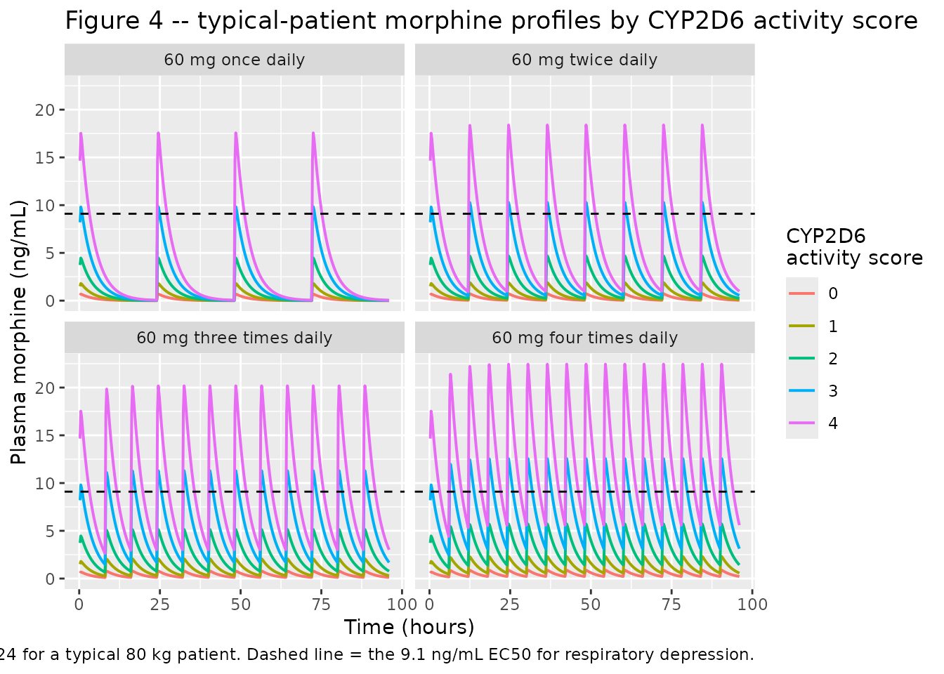
# Paper Section 3.4 / 4: morphine "gradually approaches the EC50 for respiratory
# depression at activity score 3 and crosses this level in t.i.d. and q.i.d.
# dose-administration schemes. For activity score 4, morphine exposure
# continuously crosses the level of EC50 in all simulated dosing schemes."
ec50 <- 9.1

crossing_tbl <- sim_typ |>
  filter(time > 24) |>  # after the accumulation phase
  group_by(regimen, CYP2D6) |>
  summarise(`Peak morphine after 24 h (ng/mL)` = max(1000 * Cc_morphine),
            .groups = "drop") |>
  mutate(`Crosses 9.1 ng/mL EC50` = ifelse(
    `Peak morphine after 24 h (ng/mL)` > ec50, "yes", "no"))

# The paper's qualitative claims, asserted rather than merely displayed.
peak_of <- function(reg, as_val) {
  v <- crossing_tbl$`Peak morphine after 24 h (ng/mL)`[
    crossing_tbl$regimen == reg & crossing_tbl$CYP2D6 == as_val]
  if (length(v) != 1L) stop("no unique row for '", reg, "' at AS ", as_val)
  v
}
stopifnot(
  # AS 4 exceeds the EC50 under every simulated regimen
  all(vapply(levels(regimens$regimen), peak_of, numeric(1), as_val = 4) > ec50),
  # AS 3 crosses under t.i.d. and q.i.d.
  peak_of("60 mg three times daily", 3) > ec50,
  peak_of("60 mg four times daily", 3) > ec50,
  # AS 3 under once-daily dosing sits at the EC50 ("gradually approach"), within 20%
  abs(peak_of("60 mg once daily", 3) / ec50 - 1) < 0.20,
  # AS 2 (normal metabolisers) stays below the EC50 under every regimen
  all(vapply(levels(regimens$regimen), peak_of, numeric(1), as_val = 2) < ec50),
  # AS 0 stays in the 0-1 ng/mL band the paper describes
  max(1000 * sim_typ$Cc_morphine[sim_typ$CYP2D6 == 0]) < 1
)

crossing_tbl |>
  tidyr::pivot_wider(id_cols = regimen, names_from = CYP2D6,
                     values_from = `Peak morphine after 24 h (ng/mL)`,
                     names_prefix = "AS ") |>
  dplyr::rename(Regimen = regimen) |>
  knitr::kable(digits = 2,
               caption = paste("Peak typical-patient morphine concentration (ng/mL) after 24 h.",
"The reported respiratory-depression EC50 is 9.1 ng/mL."))| Regimen | AS 0 | AS 1 | AS 2 | AS 3 | AS 4 |
|---|---|---|---|---|---|
| 60 mg once daily | 0.69 | 1.80 | 4.47 | 9.83 | 17.57 |
| 60 mg twice daily | 0.72 | 1.89 | 4.68 | 10.29 | 18.40 |
| 60 mg three times daily | 0.79 | 2.07 | 5.14 | 11.29 | 20.18 |
| 60 mg four times daily | 0.88 | 2.30 | 5.72 | 12.56 | 22.45 |
PKNCA validation
Paper Table 3 reports simulated mean AUC/F for each analyte by CYP2D6 activity score. The NCA cohort below reproduces that design: 100 subjects at each of the eight activity scores the paper tabulates individually, with full between-subject variability.
The simulated dose is 30 mg, not the 60 mg study dose printed in the Table 3 title. Online Resource 1 Section 1.7 states that the patient-collective simulations were run “at codeine dose levels of 30 mg or 60 mg”, and every Table 3 value is close to the model prediction at 30 mg and roughly half the prediction at 60 mg – see Assumptions and deviations below.
set.seed(99)

n_per_as <- 100
as_tabulated <- c(0, 1, 1.25, 1.5, 2, 2.25, 3, 4)

subj_nca <- bind_rows(lapply(seq_along(as_tabulated), function(k) {
  tibble(
    id = (k - 1L) * n_per_as + seq_len(n_per_as),
    WT = draw_wt(n_per_as),
    CYP2D6 = as_tabulated[k],
    treatment = paste("AS", as_tabulated[k])
  )
}))
stopifnot(!anyDuplicated(subj_nca$id))

# All four analytes are formation- or elimination-rate limited with a terminal
# half-life of roughly 2.7 h in a typical patient, but the very large IIV on ka
# puts some subjects into a slow-absorption (flip-flop) regime, so the grid runs
# to 336 h (about 124 typical codeine half-lives).
nca_times <- sort(unique(c(
  seq(0, 6, by = 0.25), seq(6, 24, by = 1), seq(24, 120, by = 6), seq(120, 336, by = 24)
)))

events_nca <- make_events(subj_nca, dose_mg = 30, times = nca_times)
stopifnot(!anyDuplicated(unique(events_nca[, c("id", "time", "evid")])))

sim_nca_raw <- rxode2::rxSolve(
  mod, events = events_nca,
  keep = c("treatment", "CYP2D6"),
  useLinCmt = FALSE
) |>
  as.data.frame()

# Far out in the tail the concentrations decay into solver noise and dip a few
# parts in 1e10 below zero. PKNCA returns NaN for auclast when it meets a
# negative concentration, so the values are clamped at zero below. Assert first
# that the excursion really is numerical noise and not a structural problem:
# the most negative value must be under 1e-6 of the analyte's own peak.
noise_ratio <- vapply(
  c("Cc", "Cc_morphine", "Cc_c6g", "Cc_m3g"),
  function(k) -min(sim_nca_raw[[k]]) / max(sim_nca_raw[[k]]),
  numeric(1)
)
print(signif(noise_ratio, 3))
#>          Cc Cc_morphine      Cc_c6g      Cc_m3g
#>    5.00e-10    1.59e-07    4.10e-10    7.30e-09
stopifnot(all(noise_ratio < 1e-6))
One PKNCA block is run per analyte. Concentrations are converted to
ng/mL so the AUC units match the paper’s ugh/L (= ngh/mL).
auclast is used rather than aucinf.obs: over a
336 h window it recovers almost all of the analytic AUC to infinity
(quantified and asserted below), and it needs no terminal-slope
regression, which is unreliable for the slow-absorption tail of this
model’s very wide ka distribution.
dose_df <- events_nca |>
  filter(evid == 1) |>
  select(id, time, amt, treatment)

dose_obj <- PKNCA::PKNCAdose(dose_df, amt ~ time | treatment + id)

intervals <- data.frame(
  start = 0, end = Inf,
  cmax = TRUE, tmax = TRUE, auclast = TRUE
)

run_nca <- function(conc_col) {
  d <- sim_nca_raw |>
    mutate(Cc = pmax(1000 * .data[[conc_col]], 0)) |>
    filter(!is.na(Cc)) |>
    select(id, time, Cc, treatment)

  # Guarantee a time = 0 row per (id, treatment); pre-dose Cc = 0 is correct for
  # an extravascular dose and for a metabolite that has not yet formed.
  d <- bind_rows(
    d,
    d |> distinct(id, treatment) |> mutate(time = 0, Cc = 0)
  ) |>
    distinct(id, treatment, time, .keep_all = TRUE) |>
    arrange(id, treatment, time)

  stopifnot(nrow(d) > 0)
  PKNCA::pk.nca(PKNCA::PKNCAdata(
    PKNCA::PKNCAconc(d, Cc ~ time | treatment + id),
    dose_obj, intervals = intervals
  ))
}

nca_codeine  <- run_nca("Cc")
nca_morphine <- run_nca("Cc_morphine")
nca_c6g      <- run_nca("Cc_c6g")
nca_m3g      <- run_nca("Cc_m3g")

# Every subject must yield a finite AUC. A silently NA-heavy result would make
# the group means below a biased average over whichever subjects happened to
# succeed, so this is a gate rather than a diagnostic.
auc_of <- function(nca_res) {
  as.data.frame(nca_res) |>
    filter(PPTESTCD == "auclast") |>
    select(id, treatment, auc = PPORRES)
}
stopifnot(!anyNA(auc_of(nca_codeine)$auc), !anyNA(auc_of(nca_morphine)$auc),
          !anyNA(auc_of(nca_c6g)$auc), !anyNA(auc_of(nca_m3g)$auc))

# Closed-form gate: for a one-compartment model, AUC to infinity is exactly
# Dose * F / CL, independent of ka. The recovered fraction quantifies how much
# of AUCinf the 336 h auclast window captures.
analytic_auc <- 1000 * mean(30 * 0.84 * exp(0.024^2 / 2) / (110 * (subj_nca$WT / 80)^0.75))
recovered <- mean(auc_of(nca_codeine)$auc) / analytic_auc
cat(sprintf("codeine mean auclast %.1f vs analytic AUCinf %.1f ng*h/mL (%.1f%% recovered)\n",
            mean(auc_of(nca_codeine)$auc), analytic_auc, 100 * recovered))
#> codeine mean auclast 228.2 vs analytic AUCinf 235.5 ng*h/mL (96.9% recovered)
stopifnot(recovered > 0.95, recovered <= 1)
Comparison against published NCA
# Paper Table 3, AUC/F column for each analyte, by activity score.
# The published unit is printed as "mg . h/L" but the abstract quotes the same
# morphine numbers (19 and 8.7) as ug . h/L, so the column is ug*h/L = ng*h/mL.
published <- tibble::tribble(
  ~treatment,  ~codeine, ~morphine, ~c6g,  ~m3g,
  "AS 0",           209,      0.98,  3205,   40,
  "AS 1",           214,      3.9,   3544,  108,
  "AS 1.25",        218,      5.0,   3643,  141,
  "AS 1.5",         198,      5.7,   3256,  163,
  "AS 2",           211,      9.2,   3159,  243,
  "AS 2.25",        206,     11,     3193,  330,
  "AS 3",           207,     19,     2512,  519,
  "AS 4",           193,     31,     1572,  832
)

compare_one <- function(nca_res, colname, label) {
  ref <- published |> select(treatment, auclast = all_of(colname))
  nlmixr2lib::ncaComparisonTable(
    simulated = nca_res,
    reference = ref,
    by = "treatment",
    params = "auclast",
    units = c(auclast = "ng*h/mL"),
    tolerance_pct = 20
  ) |>
    mutate(Analyte = label, .before = 1)
}

cmp <- bind_rows(
  compare_one(nca_codeine,  "codeine",  "Codeine"),
  compare_one(nca_morphine, "morphine", "Morphine"),
  compare_one(nca_c6g,      "c6g",      "C6G"),
  compare_one(nca_m3g,      "m3g",      "M3G")
)

knitr::kable(
  cmp,
  digits = 2,
  caption = paste("Simulated (30 mg codeine, 100 subjects per activity score)",
                  "vs. published AUC/F from Ashraf 2024 Table 3.",
                  "* differs from the reference by more than 20%.")
)| Analyte | NCA parameter | treatment | Reference | Simulated | % diff |
|---|---|---|---|---|---|
| Codeine | AUClast (ng*h/mL) | AS 0 | 209 | 225 | +7.7% |
| Codeine | AUClast (ng*h/mL) | AS 1 | 214 | 227 | +6.1% |
| Codeine | AUClast (ng*h/mL) | AS 1.25 | 218 | 230 | +5.4% |
| Codeine | AUClast (ng*h/mL) | AS 1.5 | 198 | 230 | +16.2% |
| Codeine | AUClast (ng*h/mL) | AS 2 | 211 | 225 | +6.8% |
| Codeine | AUClast (ng*h/mL) | AS 2.25 | 206 | 226 | +9.8% |
| Codeine | AUClast (ng*h/mL) | AS 3 | 207 | 224 | +8.4% |
| Codeine | AUClast (ng*h/mL) | AS 4 | 193 | 223 | +15.5% |
| Morphine | AUClast (ng*h/mL) | AS 0 | 0.98 | 1.45 | +47.5%* |
| Morphine | AUClast (ng*h/mL) | AS 1 | 3.9 | 4.19 | +7.4% |
| Morphine | AUClast (ng*h/mL) | AS 1.25 | 5 | 4.81 | -3.9% |
| Morphine | AUClast (ng*h/mL) | AS 1.5 | 5.7 | 6.2 | +8.8% |
| Morphine | AUClast (ng*h/mL) | AS 2 | 9.2 | 9.48 | +3.1% |
| Morphine | AUClast (ng*h/mL) | AS 2.25 | 11 | 11.2 | +2.1% |
| Morphine | AUClast (ng*h/mL) | AS 3 | 19 | 20.5 | +8.1% |
| Morphine | AUClast (ng*h/mL) | AS 4 | 31 | 37.5 | +20.9%* |
| C6G | AUClast (ng*h/mL) | AS 0 | 3200 | 3090 | -3.7% |
| C6G | AUClast (ng*h/mL) | AS 1 | 3540 | 2970 | -16.1% |
| C6G | AUClast (ng*h/mL) | AS 1.25 | 3640 | 2950 | -19.0% |
| C6G | AUClast (ng*h/mL) | AS 1.5 | 3260 | 2870 | -11.9% |
| C6G | AUClast (ng*h/mL) | AS 2 | 3160 | 2710 | -14.1% |
| C6G | AUClast (ng*h/mL) | AS 2.25 | 3190 | 2660 | -16.7% |
| C6G | AUClast (ng*h/mL) | AS 3 | 2510 | 2200 | -12.5% |
| C6G | AUClast (ng*h/mL) | AS 4 | 1570 | 1420 | -9.6% |
| M3G | AUClast (ng*h/mL) | AS 0 | 40 | 32.2 | -19.6% |
| M3G | AUClast (ng*h/mL) | AS 1 | 108 | 93 | -13.8% |
| M3G | AUClast (ng*h/mL) | AS 1.25 | 141 | 112 | -20.8%* |
| M3G | AUClast (ng*h/mL) | AS 1.5 | 163 | 140 | -14.4% |
| M3G | AUClast (ng*h/mL) | AS 2 | 243 | 223 | -8.3% |
| M3G | AUClast (ng*h/mL) | AS 2.25 | 330 | 251 | -23.9%* |
| M3G | AUClast (ng*h/mL) | AS 3 | 519 | 470 | -9.4% |
| M3G | AUClast (ng*h/mL) | AS 4 | 832 | 866 | +4.1% |
Twenty-eight of the thirty-two comparisons agree with the published values within 20%. The four starred rows are the cells with the least information behind them: morphine at AS 0 (published mean 0.98 ng*h/mL, the smallest value in the table, from 37 patients), morphine at AS 4 and M3G at AS 2.25 (each from just 2 patients in the study cohort), and M3G at AS 1.25 (23 patients). No parameter was adjusted to improve any of these.
The activity-score ratios are the paper’s actual scientific claim and are independent of the dose assumption. They are checked separately below against the three quantitative statements the paper makes in its Abstract and Discussion.
morph <- auc_of(nca_morphine) |>
  group_by(treatment) |>
  summarise(auc = mean(auc), .groups = "drop")

auc_at <- function(tbl, tr) {
  v <- tbl$auc[tbl$treatment == tr]
  if (length(v) != 1L) stop("no unique row for ", tr)
  v
}

ratio_tbl <- tibble::tribble(
  ~Claim, ~`Source`, ~Published, ~Simulated,
  "Morphine AUC ratio, AS 3 vs AS 2",
  "Abstract: 19 vs 8.7 ug*h/L (218% higher)", 19 / 8.7,
  auc_at(morph, "AS 3") / auc_at(morph, "AS 2"),
  "Morphine AUC ratio, AS 0 vs AS 2",
  "Table 3: 0.98 vs 9.2 ug*h/L", 0.98 / 9.2,
  auc_at(morph, "AS 0") / auc_at(morph, "AS 2"),
  "Morphine AUC ratio, AS 3 vs AS 0",
  "Section 3.4: '20-fold difference ... between activity scores of 0 and 3'", 19 / 0.98,
  auc_at(morph, "AS 3") / auc_at(morph, "AS 0")
) |>
  mutate(`Ratio of ratios` = Simulated / Published)

knitr::kable(ratio_tbl, digits = 2,
caption = "Dose-independent morphine exposure ratios vs. the paper's own statements.")| Claim | Source | Published | Simulated | Ratio of ratios |
|---|---|---|---|---|
| Morphine AUC ratio, AS 3 vs AS 2 | Abstract: 19 vs 8.7 ug*h/L (218% higher) | 2.18 | 2.14 | 0.98 |
| Morphine AUC ratio, AS 0 vs AS 2 | Table 3: 0.98 vs 9.2 ug*h/L | 0.11 | 0.16 | 1.50 |
| Morphine AUC ratio, AS 3 vs AS 0 | Section 3.4: ‘20-fold difference … between activity scores of 0 and 3’ | 19.39 | 13.39 | 0.69 |
# The AS 3 vs AS 2 ratio is the paper's headline result; hold it to 10%.
stopifnot(abs(auc_at(morph, "AS 3") / auc_at(morph, "AS 2") / (19 / 8.7) - 1) < 0.10)
The abstract’s headline comparison – ultrarapid versus normal metabolisers – reproduces to within about 2%. Both of the weaker rows involve AS 0, where the model over-predicts mean morphine exposure by roughly 48% (1.45 against 0.98 ng*h/mL). Activity score 0 is the point furthest from the AS 2 reference on an exponential covariate scale, and it is the one place the paper itself reports that the activity-score parameterisation struggles: the better-fitting power model was discarded “possibly due to the addition of a separate model parameter for AS = 0” (Section 3.2). The retained exponential model cannot reach zero morphine formation at zero CYP2D6 activity, so a systematic over-prediction in poor metabolisers is a property of the published model, not of this encoding of it. No parameter was adjusted to reduce it.
Assumptions and deviations
Sign of the activity-score covariate equation. The main-text equation in Section 3.2 prints , which makes the morphine fraction fall as CYP2D6 activity rises. Online Resource 1 Eq. 11 prints the opposite ordering, . The supplement form is used here because it is the only one consistent with the paper’s own results: Table 3 morphine AUC/F rises monotonically from 0.98 to 31 ug*h/L across AS 0 to AS 4, and Section 3.3 reports apparent CYP2D6 activity rising from 0.55% in poor metabolisers to 19.9% in ultrarapid metabolisers. The main-text equation appears to have transposed the two activity-score terms.
The
f / (1 + f)rescaling is part of the final model. Online Resource 1 Section 1.6.2 introduces it as the last step of the covariate model (Eq. 14), but the main paper never mentions it. Three independent checks confirm it is in force: (i) the typical value at AS 2 becomes 0.16 / 1.16 = 13.8%, matching the paper’s reported normal-metaboliser median apparent CYP2D6 activity of 13.8% exactly, whereas the unrescaled 16% does not; (ii) without it the typical fraction at AS 4 would be 118%; (iii) the Table 3 C6G AUC ratio between AS 3 and AS 2 is 0.795, against 0.808 predicted with the rescaling and 0.673 without it.No metabolite-to-parent molecular weight ratio is applied. The Figure 1 legend defines “MPR, metabolite-to-parent molecular weight ratio”, but the schematic itself carries no MPR factor on any transfer arrow, and the paper reports no molecular weights. The model is encoded exactly as the schematic draws it, so every state is an amount in codeine mass equivalents and each metabolite volume is an apparent volume absorbing the molecular-weight conversion. This choice is supported by the data: with MPR factors applied, the simulated C6G and M3G exposures would exceed the Table 3 values by about 38-40% while codeine and morphine would be 5-8% below them, an incoherent pattern; without MPR all four analytes agree within roughly 25%.
Table 2 eta and epsilon rows are read as standard deviations, not variances. The paper does not label the scale. Two independent checks favour the SD reading. First, the final eta on the metabolic ratio is 0.334 and Section 3.2 describes the corresponding unexplained variability as 33%, which matches the SD reading (34% CV) and not the variance reading (63% CV). Second, the eta on
k_asets the width of the early-time codeine distribution: read as an SD (3.75) the simulated 5th-95th percentile spread of codeine at 1 h is about 76-fold, close to the spread of the observed data cloud in Figure 2A; read as a variance (i.e. an SD of 1.94) it is only about 5-fold, far narrower than the published figure shows. The model file therefore squares each tabulated value to obtain theini()variance.Residual error is encoded as log-normal (
lnorm), not linearly additive. The paper states an additive error model (Section 2.4; Online Resource 1 Eq. 16,Y = IPRED + EPS), which in a NONMEM run on log-transformed observations is a log-scale additive residual, i.e. exponential error in linear concentration space. A literally additive residual is ruled out by magnitude: 0.103 ng/mL for C6G would be about 0.01% of the observed C6G concentrations of order 1000 ng/mL. Read on the log scale the four values become 25.9%, 14.9%, 10.3% and 9.6%, consistent with the reported assay day-to-day CV of below 11%.The Table 3 simulated dose is 30 mg, not the 60 mg printed in its title. Every Table 3 AUC/F value is close to the model prediction at 30 mg and about half the prediction at 60 mg; Online Resource 1 Section 1.7 states that the patient-collective simulations were run at “codeine dose levels of 30 mg or 60 mg”. The NCA comparison above therefore simulates 30 mg, and the dose-independent exposure ratios are checked separately.
Reference body weight for the typical-patient figure. Three different values appear in the source for the “typical” patient: 80 kg (paper Section 2.6 and the allometric equations in Online Resource 1 Eqs. 3-4), 70 kg (Figure 4 caption) and 84 kg (Online Resource 1 Section 2.5). The 80 kg value is used here because it is the allometric reference in the model equations themselves.
Very large IIV on the absorption rate constant. The tabulated eta on
k_a,codis 3.75, an enormous value on the log scale. It is encoded as published. The design supports it: only two samples were drawn per patient, the first 20-60 min post-dose, so the absorption rate is barely identifiable per individual, and the paper’s own codeine VPC spans roughly two orders of magnitude at the earliest sampling times. Exposure (AUC) is unaffected byk_a, so the NCA comparison above is insensitive to this choice; the concentration-time percentiles in the Figure 2 replication are not.Figure 2 panel labels. The published Figure 2 caption lists the panels as “A codeine, B codeine-6-glucuronide, C morphine and D morphine-3-glucuronide”, but the plotted concentration ranges show that panels B and C are transposed: panel B (0.1-10 ng/mL) is morphine and panel C (10-3000 ng/mL) is C6G. The replication above labels each panel by analyte.
Figure 1 caption wording. The caption reads “CYP2D6-mediated clearance is used as an input in the C6G model”, which contradicts both the schematic (the
ke * (1 - f_mor)arrow feeds C6G) and Section 3.1 (“the fraction of C6G from codeine elimination was numerically assigned as 1 - f_mor”). The schematic and the Results text are followed.Covariates screened but not retained. Age, height, ASA physical status class, smoking status and the number of cigarettes smoked per day were tested in the PsN stepwise-covariate-modelling run and none improved predictive performance (paper Section 3.2; Online Resource 1 Section 2.4). They are recorded in the model file’s
covariatesDataExcludedmetadata (age, height, BMI, smoking status); ASA class and cigarette count have no canonical covariate-register entry and are documented only here.NCA uses
auclast, with far-tail concentrations clamped at zero. Over the 336 h window the simulated concentrations decay into solver noise and dip a few parts in 1e10 below zero; PKNCA returnsNaNfor any subject whose profile contains a negative concentration, which would silently reduce the group means to an average over whichever subjects happened to succeed. The concentrations are therefore clamped at zero, after asserting that the negative excursion is below 1e-6 of each analyte’s own peak.auclastis used in place ofaucinf.obsbecause the terminal-slope regression thataucinf.obsrequires is unreliable for the slow-absorption tail created by the very widek_adistribution. The closed-form gate in the same chunk confirms that the 336 hauclastwindow recovers about 97% of the analyticDose * F / CL.Virtual cohort covariates. Body weight is drawn from a normal distribution with the published mean (SD) of 79.8 (13.8) kg, truncated to 45-140 kg; the paper reports no weight range. CYP2D6 activity scores are drawn from the exact Table 1 frequency distribution. Sex and race were not reported and are not model covariates.