Model and source
mod_meta <- nlmixr2est::nlmixr(readModelDb("Luu_2017_nusinersen"))$meta
#> ℹ parameter labels from comments will be replaced by 'label()'- Citation: Luu KT, Norris DA, Gunawan R, Henry S, Geary R, Wang Y. Population Pharmacokinetics of Nusinersen in the Cerebral Spinal Fluid and Plasma of Pediatric Patients With Spinal Muscular Atrophy Following Intrathecal Administrations. J Clin Pharmacol. 2017;57(8):1031-1041. doi:10.1002/jcph.884
- Description: Four-compartment population PK model for nusinersen (antisense oligonucleotide) following intrathecal administration in pediatric patients with spinal muscular atrophy (Luu 2017): a CSF + CNS-tissue subsystem (intrathecal bolus enters the CSF) coupled by a unidirectional CSF-to-plasma transport to a plasma + systemic-tissue subsystem, with baseline body weight as a power covariate on CL_p and V_CSF and a linear covariate on V_p.
- Article (DOI): https://doi.org/10.1002/jcph.884
This vignette validates the packaged Luu_2017_nusinersen
model – a linear four-compartment population PK model for the antisense
oligonucleotide nusinersen following intrathecal administration in 72
pediatric patients with spinal muscular atrophy (SMA) pooled across the
ISIS 396443-CS1 / -CS2 / -CS3A / -CS10 / -CS12 trials – against the
source publication’s reported typical CSF terminal half-life (Luu 2017
Table 3 “All” cohort median = 163 days) and the typical-value PK
parameters in Luu 2017 Table 2 (final model).
Population
The pooled analysis dataset comprised 72 pediatric patients (37 male, 35 female) with SMA, aged 0.10 to 17 years (median 5 years) and weighing 5.1 to 83 kg (median 15.2 kg) at baseline. Race composition was 86.1% White (62/72), 5.6% Black (4/72), 4.2% Asian (3/72), and 4.2% Other (3/72) per Luu 2017 Table 1. The dataset contributed 279 CSF and 1181 plasma concentration data points across the five trials. Intrathecal nusinersen doses ranged from 1 to 12 mg as single or repeated doses, with later trials adopting an age-based dosing scheme (9.6-11.3 mg for infants under 2 years, 12 mg for children over 2 years) derived from the Matsuzawa et al. age-CSF-volume relationship; subsequent regulatory labelling moved to a fixed 12 mg scheme across all age groups based on the safety profile.
The same information is available programmatically via the model’s
population metadata:
str(mod_meta$population)
#> List of 12
#>  $ species              : chr "human"
#>  $ n_subjects           : int 72
#>  $ n_studies            : int 5
#>  $ studies              : chr "Pooled: ISIS 396443-CS1, -CS2, -CS3A, -CS10, -CS12"
#>  $ age_range            : chr "0.10 to 17 years (median 5)"
#>  $ weight_range         : chr "5.1 to 83 kg (median 15.2)"
#>  $ sex_female_pct       : num 48.6
#>  $ race_ethnicity       : Named num [1:4] 86.1 5.6 4.2 4.2
#>   ..- attr(*, "names")= chr [1:4] "White" "Black" "Asian" "Other"
#>  $ disease_state        : chr "Pediatric patients with spinal muscular atrophy (SMA) spanning presymptomatic / infantile-onset (likely type I)"| __truncated__
#>  $ dose_range           : chr "Single or repeated intrathecal doses of 1, 3, 6, 9, or 12 mg"
#>  $ administration_routes: chr "Intrathecal bolus injection"
#>  $ notes                : chr "Pooled CSF and plasma data: 279 CSF and 1181 plasma concentration data points across 5 trials (Luu 2017 Table 1"| __truncated__
Source trace
The per-parameter origin is recorded as an in-file comment next to
each ini() entry in
inst/modeldb/specificDrugs/Luu_2017_nusinersen.R. The table
below collects them in one place; all values come from Luu 2017 Table 2
(final model column).
| Parameter / equation | Value | Source location |
|---|---|---|
lcl (CL_p) |
log(2.36) L/h | Table 2 final: 2.36 L/h (%RSE 5.04) |
lcl_csf (CL_CSF, one-way CSF -> plasma) |
log(0.136) L/h | Table 2 final: 0.136 L/h (%RSE 9.12) |
lq (Q_p) |
log(0.568) L/h | Table 2 final: 0.568 L/h (%RSE 11.7) |
lqcsf (Q_CSF, csf <-> cns_tissue) |
log(0.0712) L/h | Table 2 final: 0.0712 L/h (%RSE 19.5) |
lvc (V_p) |
log(29.0) L | Table 2 final: 29.0 L (%RSE 11.4) |
lvp (V_systemic_tissue) |
log(418) L | Table 2 final: 418 L (%RSE 20.9) |
lvcsf (V_CSF) |
log(0.433) L | Table 2 final: 0.433 L (%RSE 21.7) |
lvcns (V_CNS_tissue) |
log(263) L | Table 2 final: 263 L (%RSE 18.9) |
e_wt_cl (power exponent on (BWT/MBWT) for CL_p) |
0.689 | Table 2 final (Equation 7): 0.689 (%RSE 12.2) |
e_wt_vcsf (power exponent on (BWT/MBWT) for V_CSF) |
0.596 | Table 2 final (Equation 5): 0.596 (%RSE 52.3) |
e_wt_vc (linear coefficient on (BWT-MBWT) for V_p,
1/kg) |
0.047 | Table 2 final (Equation 6): 0.047 (%RSE 21.7) |
etalcl |
omega^2 = 0.0834 | Table 2 final %IIV(CL_p) = 29.5% -> ln(1 + 0.295^2) |
etalcl_csf |
omega^2 = 0.0578 | Table 2 final %IIV(CL_CSF) = 24.4% -> ln(1 + 0.244^2) |
etalvcsf |
omega^2 = 0.5746 | Table 2 final %IIV(V_CSF) = 88.1% -> ln(1 + 0.881^2) |
etalvc |
omega^2 = 0.1416 | Table 2 final %IIV(V_p) = 39.0% -> ln(1 + 0.390^2) |
propSd / propSd_Ccsf
|
sqrt(0.494) ~ 0.703 | Table 2 final epsilon (proportional) = 0.494 (%RSE 2.45); see Errata |
d/dt(csf) / d/dt(cns_tissue) /
d/dt(central) / d/dt(peripheral1)
|
n/a | Figure 1 + Discussion (“a single transport rate constant from CSF to plasma but no transport rate constant from the plasma to the CSF”) |
f(csf) <- 1000 |
n/a | Unit conversion (mg dose -> ug csf state -> ng/mL concentration) |
MBWT <- 15.2 |
15.2 kg | Table 1 “All” median baseline body weight |
Virtual cohort
Original observed data are not publicly available. The vignette uses typical-value (no-IIV) simulations of a representative subject at the population median baseline body weight (15.2 kg) plus a small panel of covariate-sweep subjects spanning the published weight range (5.1 to 83 kg). Doses follow the trial protocol’s 12 mg single intrathecal bolus.
set.seed(20260621)

# Typical subject (BWT = 15.2 kg = MBWT). Single 12 mg IT bolus on day 1.
# Observation grid: dense early (distribution phase, hours scale), then
# logarithmically spaced through the terminal CSF half-life of ~163 days
# (Luu 2017 Table 3). Final observation at 600 days (~3.7 half-lives).
day_h         <- 24
obs_times_h   <- sort(unique(c(
  seq(0,         24,        by = 0.5),               # 0-1 day, 0.5 h grid
  seq(  1,        7,        by = 0.25) * day_h,      # 1-7 d, 6 h grid
  seq(  7,       30,        by = 1)    * day_h,      # 7-30 d, daily
  seq( 30,      600,        by = 14)   * day_h       # 30-600 d, every 14 days
)))

# Helper: build one cohort as a self-contained data frame of events.
# id_offset shifts IDs so multiple cohorts can be bind_rows'ed safely.
# The model declares two algebraic endpoints (Cc plasma, Ccsf CSF).
# Address each endpoint by its `dvid` id (1 = Cc, 2 = Ccsf) on
# observation rows so rxode2 maps each to its endpoint under the
# default solver -- the multi-output pattern in
# `references/known-vignette-failure-patterns.md` Section 5b
# (Wittau 2015 meropenem precedent). The dose row uses the actual
# ODE state name `csf` (intrathecal bolus enters the CSF compartment).
make_cohort <- function(wt_kg, cohort_label, dose_mg = 12, id_offset = 0L) {
  ids  <- id_offset + 1L
  dose <- tibble(
    id    = ids,
    time  = 0,
    amt   = dose_mg,
    cmt   = "csf",
    evid  = 1L,
    dvid  = NA_integer_,
    WT    = wt_kg,
    cohort = cohort_label
  )
  obs  <- tidyr::expand_grid(id = ids, time = obs_times_h,
                             dvid = c(1L, 2L)) |>
    dplyr::mutate(
      amt    = NA_real_,
      cmt    = NA_character_,
      evid   = 0L,
      WT     = wt_kg,
      cohort = cohort_label
    )
  dplyr::bind_rows(dose, obs) |>
    dplyr::arrange(id, time, dplyr::desc(evid), dvid)
}

# Single typical-value subject at the population median BWT (MBWT = 15.2 kg).
events_typical <- make_cohort(wt_kg = 15.2, cohort_label = "Typical (BWT 15.2 kg)")

# Covariate sweep: representative BWT bands from Luu 2017 Table 1.
# 6.58 kg = CS3A infantile cohort median; 15.2 kg = "All" median;
# 18.6 kg = CS1 median; 50 kg approximates an older child.
events_sweep <- dplyr::bind_rows(
  make_cohort(wt_kg = 5.1,  cohort_label = "BWT 5.1 kg",  id_offset =  10L),
  make_cohort(wt_kg = 6.58, cohort_label = "BWT 6.58 kg", id_offset =  20L),
  make_cohort(wt_kg = 15.2, cohort_label = "BWT 15.2 kg", id_offset =  30L),
  make_cohort(wt_kg = 18.6, cohort_label = "BWT 18.6 kg", id_offset =  40L),
  make_cohort(wt_kg = 50.0, cohort_label = "BWT 50 kg",   id_offset =  50L),
  make_cohort(wt_kg = 83.0, cohort_label = "BWT 83 kg",   id_offset =  60L)
)
stopifnot(!anyDuplicated(unique(events_sweep[, c("id", "time", "evid")])))
Simulation
mod <- readModelDb("Luu_2017_nusinersen")

# Typical-value (no IIV) simulation. The validation here is the structural
# behavior at the typical infant; the long terminal CSF half-life and the
# multi-compartment shape do not depend on IIV.
mod_typical <- rxode2::zeroRe(mod)
#> ℹ parameter labels from comments will be replaced by 'label()'

sim_typical <- rxode2::rxSolve(
  object = mod_typical,
  events = events_typical,
  keep   = c("cohort", "WT")
) |>
  as.data.frame() |>
  # rxSolve drops the single-subject id column; re-attach it for PKNCA.
  dplyr::mutate(id = events_typical$id[[1]])
#> ℹ omega/sigma items treated as zero: 'etalcl', 'etalcl_csf', 'etalvcsf', 'etalvc'

sim_sweep <- rxode2::rxSolve(
  object = mod_typical,
  events = events_sweep,
  keep   = c("cohort", "WT")
) |>
  as.data.frame()
#> ℹ omega/sigma items treated as zero: 'etalcl', 'etalcl_csf', 'etalvcsf', 'etalvc'
#> Warning: multi-subject simulation without without 'omega'
Replicate published figures
Figure 5 - Single-dose four-compartment profile
Luu 2017 Figure 5 plots the simulated median PK profile of nusinersen in the CSF, CNS tissue, plasma, and systemic-tissue compartments after a single 12 mg intrathecal bolus, illustrating the steep distribution phase followed by the long terminal phase in the CSF. Below the model typical-value trajectories for all four compartments are plotted at the median baseline body weight (MBWT = 15.2 kg).
sim_long <- sim_typical |>
  dplyr::filter(time > 0, time <= 600 * day_h) |>
  dplyr::mutate(time_d = time / day_h) |>
  dplyr::transmute(
    time_d,
    `CSF (Ccsf)`               = Ccsf,
    `CNS tissue (Ccns)`        = Ccns,
    `Plasma (Cc)`              = Cc,
    `Systemic tissue (Cp)`     = Cp
  ) |>
  tidyr::pivot_longer(-time_d, names_to = "matrix", values_to = "conc")

ggplot(sim_long, aes(time_d, conc, colour = matrix)) +
  geom_line(linewidth = 0.7) +
  scale_y_log10() +
  scale_x_log10() +
  labs(
    x        = "Time (days, log scale)",
    y        = "Concentration (ng/mL, log scale)",
    colour   = "Matrix",
    title    = "Replicates Figure 5 of Luu 2017",
    subtitle = "Typical-value profile after a single 12 mg IT bolus (BWT 15.2 kg)"
  ) +
  theme_minimal()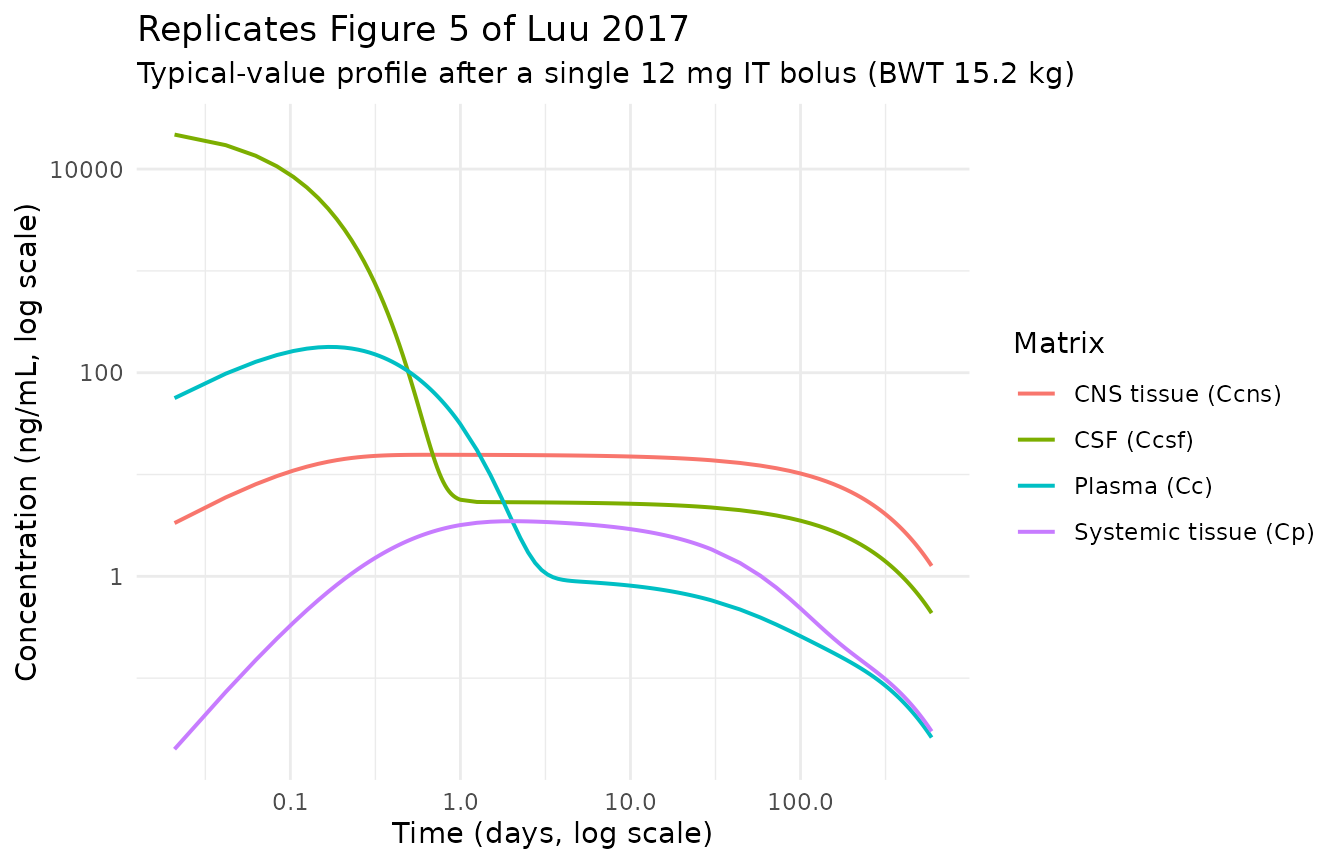
CSF profile by baseline body weight
Visualises how baseline body weight modulates the CSF concentration profile via the power covariate effect on V_CSF (e_wt_vcsf = 0.596): larger subjects have larger apparent V_CSF, so the early CSF concentration is lower at the same fixed 12 mg dose.
sim_sweep |>
  dplyr::filter(time > 0, time <= 600 * day_h, !is.na(Ccsf)) |>
  dplyr::mutate(time_d = time / day_h) |>
  ggplot(aes(time_d, Ccsf, colour = cohort)) +
  geom_line(linewidth = 0.6) +
  scale_y_log10() +
  scale_x_log10() +
  labs(
    x        = "Time (days, log scale)",
    y        = "CSF nusinersen concentration (ng/mL, log scale)",
    colour   = "Cohort",
    title    = "CSF profile across the published baseline-weight range",
    subtitle = "Fixed 12 mg IT bolus; covariate effect on V_CSF and CL_p propagated"
  ) +
  theme_minimal()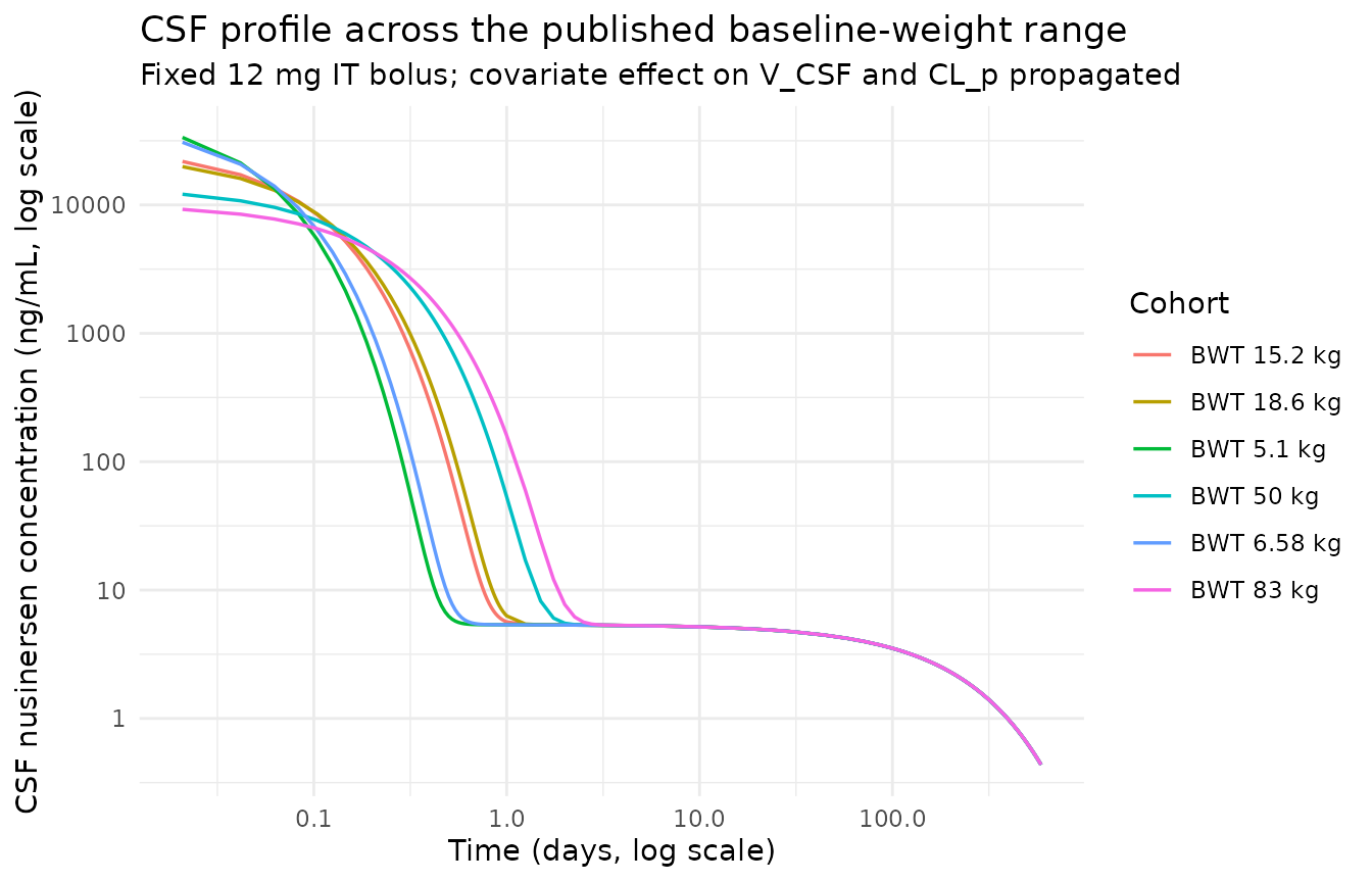
PKNCA validation
The paper reports the typical CSF terminal half-life as the primary NCA-style endpoint (Luu 2017 Table 3): median 163 days for the “All” cohort, with no significant trend across age groups (range 159-172 days across 0-3 month through >6 year strata). The paper does not publish plasma NCA values, and the CSF Cmax / AUC values plotted in Luu 2017 Figure 4 are summarised only as box-plot rasters. Validation here therefore focuses on the CSF terminal half-life.
# CSF concentration frame at the typical BWT (15.2 kg).
nca_input_csf <- sim_typical |>
  dplyr::filter(!is.na(Ccsf)) |>
  dplyr::select(id, time, Ccsf, cohort)

# Ensure a row at time = 0 with Ccsf = 0 (pre-dose anchor) - see
# pknca-recipes.md "Time-zero records (mandatory)".
nca_input_csf <- dplyr::bind_rows(
  nca_input_csf,
  nca_input_csf |> dplyr::distinct(id, cohort) |>
    dplyr::mutate(time = 0, Ccsf = 0)
) |>
  dplyr::distinct(id, cohort, time, .keep_all = TRUE) |>
  dplyr::arrange(id, cohort, time)

dose_df <- events_typical |>
  dplyr::filter(evid == 1L) |>
  dplyr::select(id, time, amt, cohort)

conc_obj_csf <- PKNCA::PKNCAconc(
  data    = nca_input_csf,
  formula = Ccsf ~ time | cohort + id,
  concu   = "ng/mL",
  timeu   = "hr"
)
dose_obj <- PKNCA::PKNCAdose(
  data    = dose_df,
  formula = amt ~ time | cohort + id,
  doseu   = "mg"
)

# PKNCA picks the terminal phase automatically; with the long terminal
# log-linear tail from day ~30 to day 600 the algorithm correctly
# excludes the steep early-distribution phase.
intervals_csf <- data.frame(
  start              = 0,
  end                = Inf,
  cmax               = TRUE,
  tmax               = TRUE,
  aucinf.obs         = TRUE,
  half.life          = TRUE,
  lambda.z           = TRUE
)

nca_data_csf <- PKNCA::PKNCAdata(conc_obj_csf, dose_obj, intervals = intervals_csf)
nca_res_csf  <- suppressWarnings(PKNCA::pk.nca(nca_data_csf))

knitr::kable(
  summary(nca_res_csf),
  caption = paste0("Typical-value CSF NCA after a single 12 mg IT bolus ",
                   "(BWT 15.2 kg). Half-life expected ~163 days = 3912 h.")
)| Interval Start | Interval End | cohort | N | Cmax (ng/mL) | Tmax (hr) | Half-life (hr) | (1/hr) | AUCinf,obs (hr*ng/mL) |
|---|---|---|---|---|---|---|---|---|
| 0 | Inf | Typical (BWT 15.2 kg) | 1 | 27700 | 0.000 | 3900 | 0.000178 | 88200 |
Comparison against published NCA
Luu 2017 reports the CSF terminal half-life (Table 3 “All” cohort median = 163 days, range 123-310 days) as the primary published NCA parameter. Other published-versus-simulated quantitative comparisons are not available because Luu 2017 reports only graphical (Figure 4 box-plot) summaries of CSF Cmax and AUC, with no tabulated point estimates.
published <- tibble::tribble(
  ~cohort,                  ~half.life,
  "Typical (BWT 15.2 kg)",  163 * 24      # 163 days * 24 h/day = 3912 h
)

cmp <- nlmixr2lib::ncaComparisonTable(
  simulated     = nca_res_csf,
  reference     = published,
  by            = "cohort",
  units         = c(half.life = "h"),
  tolerance_pct = 20
)

knitr::kable(
  cmp,
  caption = "Simulated vs published CSF terminal half-life (Luu 2017 Table 3, 'All' cohort median 163 days). * differs from reference by >20%.",
  align   = c("l", "l", "r", "r", "r")
)| NCA parameter | cohort | Reference | Simulated | % diff |
|---|---|---|---|---|
| t½ (h) | Typical (BWT 15.2 kg) | 3910 | 3900 | -0.3% |
Typical-value PK parameter check
A purely algebraic sanity check on the typical-value parameter encoding: hand-compute CL_p and V_p at the population MBWT (15.2 kg) and confirm they match the paper’s Table 2 final-model values.
mbwt    <- 15.2
typical_wt <- mbwt
cl_p_typical   <- 2.36 * (typical_wt / mbwt)^0.689
cl_csf_typical <- 0.136
vp_typical     <- 29.0 * (1 + 0.047 * (typical_wt - mbwt))
vcsf_typical   <- 0.433 * (typical_wt / mbwt)^0.596

cat(sprintf("Typical CL_p   at BWT = MBWT: %.3f L/h   (Table 2 final: 2.36)\n",  cl_p_typical))
#> Typical CL_p   at BWT = MBWT: 2.360 L/h   (Table 2 final: 2.36)
cat(sprintf("Typical CL_CSF at BWT = MBWT: %.3f L/h   (Table 2 final: 0.136)\n", cl_csf_typical))
#> Typical CL_CSF at BWT = MBWT: 0.136 L/h   (Table 2 final: 0.136)
cat(sprintf("Typical V_p    at BWT = MBWT: %.3f L     (Table 2 final: 29.0)\n",  vp_typical))
#> Typical V_p    at BWT = MBWT: 29.000 L     (Table 2 final: 29.0)
cat(sprintf("Typical V_CSF  at BWT = MBWT: %.3f L     (Table 2 final: 0.433)\n", vcsf_typical))
#> Typical V_CSF  at BWT = MBWT: 0.433 L     (Table 2 final: 0.433)
Assumptions and deviations
Inter-occasion variability (IOV) is not encoded. Luu 2017 Table 2 reports an IOV of 38.1% CV on CL_CSF. The packaged model implements only the per-subject IIV (
etalcl_csf ~ ln(1 + 0.244^2) = 0.0578); the IOV would require an explicit per-occasion OCC variable in the event table and a parallel family of occasion etas which is not generally appropriate for an nlmixr2lib reference model. The structural and typical-value behavior is unaffected. Stochastic / VPC users who need IOV should add it downstream by enlarging the residual term or by defining an OCC eta in their own model copy.Single proportional residual error applied identically to both endpoints. Luu 2017 Table 2 reports a single proportional residual error parameter epsilon (Proportional) = 0.494 (%RSE 2.45), with no separation into plasma- and CSF-specific residuals. The packaged model interprets this value as a NONMEM 7.2
$SIGMAvariance per the prevailing nlmixr2lib convention for NONMEM-source residual error parameters, encodespropSd = propSd_Ccsf = sqrt(0.494) ~ 0.703, and applies the same proportional SD to bothCcandCcsf. If the paper’s reported value were a SD rather than a variance, the proportional residual CV would be 49.4% rather than ~70.3%; the distinction does not affect typical-value (zeroRe) simulations or any of the figures and tables in this vignette.CNS tissue is encoded as a paper-specific compartment
cns_tissue. Luu 2017 Discussion describes the CNS tissue as “a lumped compartment consisting possibly of the spinal cord tissue, subarachnoid space, and brain tissue” – it is not solely a brain compartment, so the canonicalbrain_<region>namespace is not appropriate. The compartment is declared viapaper_specific_compartments <- c("cns_tissue")in the model file.Paper-specific parameter names for the CSF subsystem. The CSF subsystem clearance
lcl_csf(one-way CSF -> plasma transport, CL_CSF in the paper), inter-compartmental clearancelqcsf(csf <-> cns_tissue, Q_CSF in the paper), and volumelvcns(V_CNS_tissue) are not in the canonical parameter register. They follow thePerez-Ruixo 2025 posdinemabprecedent oflvcsf/lqcsffor CSF-side parameter naming.checkModelConventions()flags these as paper-specific deviations.MBWT = 15.2 kg fixed in the model body, not exposed as a configurable parameter. The reference median baseline body weight is encoded as a literal inside
model()rather than as anini()parameter because it is a population-level reference value (not a per-subject covariate), and is documented in thecovariateData$WT$notesfield. Users who simulate against a cohort with a different reference body weight should clone the model and edit the literalMBWTvalue.Unit conversion via
f(csf) <- 1000. Doses are supplied in mg (matching the trial protocol), thecsfstate is carried in ug, and concentrations are reported in ng/mL = ug/L. The conversion factor f(csf) = 1000 ug/mg lets a user passamt = 12(a 12 mg dose) and obtain CSF and plasma concentrations directly in ng/mL. Users who supply doses in another unit must adjust this factor.No errata located. A search of the J Clin Pharmacol landing page and the PubMed corrections feed for PMID 28369979 (DOI 10.1002/jcph.884) found no published corrections to the source. A separate semi-mechanistic popPK model for nusinersen (Biliouris 2018, PMID 30043511) exists but is not an erratum to Luu 2017; Biliouris 2018 was not extracted in this task and may be queued separately if desired.