mRNA-6231 (Liric Rajlic 2024)
Source:vignettes/articles/LiricRajlic_2024_mRNA6231.Rmd
LiricRajlic_2024_mRNA6231.RmdModel and source
- Citation: Liric Rajlic I, Rong Y, Gaffney M, Faya P, Sun J, Liu C, Huang Y, Mahajan S, Hoffmann M, Smith M, Narasimhan B, Patel N. Translational kinetic-pharmacodynamics of mRNA-6231, an investigational mRNA therapeutic encoding mutein interleukin-2. CPT Pharmacometrics Syst Pharmacol. 2024;13(6):1067-1076. doi:10.1002/psp4.13142.
- Description: Preclinical (cynomolgus monkey). Semi-mechanistic kinetic-pharmacodynamic (KPD) model for mRNA-6231, a lipid-nanoparticle-encapsulated mRNA encoding a human interleukin-2 mutein fused to human serum albumin (HSA-IL2m), given subcutaneously. The lipid-nanoparticle and mRNA are below assay quantitation, so no drug concentration is fitted: a subcutaneous depot feeds a virtual transit compartment (unit volume) whose mRNA concentration drives saturable synthesis of HSA-IL2m protein into a central compartment. Protein in the central compartment equilibrates with an empirical effect compartment, and effect-site HSA-IL2m stimulates the production rate of a one-compartment indirect-response model for the percentage of regulatory T cells (FOXP3+ of CD4+). Structural parameters carry allometric body-weight scaling (reference 2.5 kg) so the monkey fit can be forward-projected to other body weights.
- Article: CPT Pharmacometrics Syst Pharmacol. 2024;13(6):1067-1076
mRNA-6231 is a lipid-nanoparticle-encapsulated mRNA encoding a human interleukin-2 mutein fused to human serum albumin (HSA-IL2m), developed to selectively expand regulatory T cells (Tregs). Because the systemic lipid and mRNA concentrations are below assay quantitation, no drug concentration is fitted; the model is a kinetic-pharmacodynamic (dose-driven) cascade from a subcutaneous depot, through a virtual mRNA transit compartment, to saturable synthesis of HSA-IL2m protein, an effect compartment, and an indirect-response turnover model for the percentage of FOXP3+ Tregs.
Population
The model was fitted to data from three non-GLP studies in male cynomolgus monkeys (Methods, “Study design”). Study 1 (N = 16, aged 2-4 years) gave repeat subcutaneous doses of 1, 3, 6 or 10 ug/kg on Days 1, 15 and 29. Study 2 (N = 12, aged 2-4 years) gave single doses of 3 or 10 ug/kg or a flat 10 ug total dose. Study 3 (N = 16, aged 2-5 years, naive and non-naive) gave single doses of 10 or 30 ug/kg or a flat 100 ug total dose. HSA-IL2m protein was measured in plasma by ELISA and percentage Tregs (FOXP3+ of CD4+) in cryopreserved PBMCs by flow cytometry. The allometric reference body weight is 2.5 kg.
The same information is available programmatically via the model’s
population metadata
(readModelDb("LiricRajlic_2024_mRNA6231")()$population).
Source trace
The per-parameter origin is recorded as an in-file comment next to
each ini() entry in
inst/modeldb/specificDrugs/LiricRajlic_2024_mRNA6231.R. The
table below collects them in one place for review.
| Equation / parameter | Value | Source location |
|---|---|---|
d/dt(depot) (SC absorption) |
n/a | Table 2, equation 1 |
d/dt(transit1) (virtual mRNA transit) |
n/a | Table 2, equation 2 |
d/dt(central) (saturable HSA-IL2m synthesis +
elimination) |
n/a | Table 2, equation 3 |
d/dt(effect) (effect-compartment equilibration) |
n/a | Table 2, equation 4 |
d/dt(treg) (indirect-response Treg turnover) |
n/a | Table 2, equation 5 |
treg(0) = kin/kout |
n/a | Table 2, equation 6 |
| Allometric scaling of ka, CLt, Vt, V, CLIL2, IL2kp | exponents -0.25, 0.65, 1, 1, 0.85, -0.25 | Table 2, equations 7-11 |
lka (ka) |
0.0749 1/h | Table 3 |
lcl_transit (CLt) |
12.865 mL/h | Table 3 |
lvt (Vt, fixed) |
1.0 mL | Table 3 |
lvc (V) |
171.56 mL | Table 3 |
lksyn (IL2kp) |
4570.3 | Table 3 |
lkm_syn (IL2k50) |
0.1312 ug/mL | Table 3 |
lcl (CLIL2) |
1.529 mL/h | Table 3 |
lke0 (ke0) |
0.011 1/h | Table 3 |
lkin (kin-Treg) |
0.0597 %/h | Table 3 |
lkout (kout-Treg) |
0.0152 1/h | Table 3 |
lemax (Emax) |
2.84 | Table 3 |
lhill (gam) |
2.47 | Table 3 |
lec50 (EC50) |
5.08 ng/mL | Table 3 |
| IIV on IL2kp, CLIL2, kin-Treg, Emax | 51.3, 22.8, 36.5, 30.2 %CV | Table 3 |
| Proportional residual error (IL-2, Treg) | 43.4, 27.1 %CV | Table 3 |
Virtual cohort
Original observed data are not publicly available. The figures below use a virtual population of male cynomolgus monkeys at the 2.5 kg allometric reference body weight, reproducing the Study 1 multiple-dose design (doses on Days 1, 15 and 29). Between-subject variability comes from the four model IIV terms (on IL2kp, CLIL2, kin-Treg and Emax).
This is a two-endpoint model (HSA-IL2m Cc and
treg). treg is both an ODE state and an
endpoint, so the observation rows use cmt = "treg", and
rxode2 returns Cc and treg together at every
observation row.
set.seed(6231)

doses <- tibble::tibble(
  dose_lbl = factor(c("1 ug/kg", "3 ug/kg", "6 ug/kg", "10 ug/kg"),
                    levels = c("1 ug/kg", "3 ug/kg", "6 ug/kg", "10 ug/kg")),
  dose_ugkg = c(1, 3, 6, 10)
)
n_per <- 100L               # <= 200 per arm
wt_ref <- 2.5               # kg, allometric reference (individual weights not reported)
dose_days <- c(0, 14, 28)   # Days 1, 15, 29 relative to first dose
obs_h <- seq(0, 72 * 24, by = 12)

# Build event rows without tidyr::crossing() on a data frame that carries a
# factor column -- crossing() would expand the factor to all its levels and
# silently duplicate subjects. expand_grid() on plain id/time vectors, then a
# join of per-subject covariates by id, is safe.
make_cohort <- function(dl, dmgk, id_offset) {
  ids <- id_offset + seq_len(n_per)
  amt_ug <- dmgk * wt_ref
  dose_rows <- tidyr::expand_grid(id = ids, time = dose_days * 24) |>
    dplyr::mutate(evid = 1L, amt = amt_ug, cmt = "depot")
  obs_rows <- tidyr::expand_grid(id = ids, time = obs_h) |>
    dplyr::mutate(evid = 0L, amt = NA_real_, cmt = "treg")
  dplyr::bind_rows(dose_rows, obs_rows) |>
    dplyr::mutate(WT = wt_ref, dose_lbl = dl) |>
    dplyr::select(id, time, evid, amt, cmt, WT, dose_lbl) |>
    dplyr::arrange(id, time, dplyr::desc(evid))
}

events <- dplyr::bind_rows(lapply(seq_len(nrow(doses)), function(i) {
  make_cohort(doses$dose_lbl[i], doses$dose_ugkg[i], id_offset = (i - 1L) * n_per)
}))
stopifnot(!anyDuplicated(unique(events[, c("id", "time", "evid")])))
Simulation
mod <- readModelDb("LiricRajlic_2024_mRNA6231")
# Structural + between-subject variability (IPRED); residual error is left off
# so the bands below are a model-prediction VPC. useLinCmt = FALSE because the
# synthesis cascade is not a linear-compartment model.
sim <- rxode2::rxSolve(mod, events = events,
  sigma = NA, useLinCmt = FALSE,
  keep = c("dose_lbl"), returnType = "data.frame")
#> ℹ parameter labels from comments will be replaced by 'label()'
Replicate published figures
# Replicates Figure 2a of Liric Rajlic 2024: multiple-dose HSA-IL2m in plasma.
sim |>
  dplyr::filter(!is.na(Cc), Cc > 0) |>
  dplyr::group_by(dose_lbl, time) |>
  dplyr::summarise(
    Q05 = quantile(Cc, 0.05), Q50 = quantile(Cc, 0.50),
    Q95 = quantile(Cc, 0.95), .groups = "drop"
  ) |>
  ggplot(aes(time / 24, Q50, colour = dose_lbl, fill = dose_lbl)) +
  geom_ribbon(aes(ymin = Q05, ymax = Q95), alpha = 0.15, colour = NA) +
  geom_line() +
  scale_y_log10() +
  labs(x = "Time (days)", y = "HSA-IL2m (ng/mL)", colour = "Dose", fill = "Dose",
       title = "Figure 2a - multiple-dose HSA-IL2m",
       caption = "Replicates Figure 2a of Liric Rajlic 2024 (Days 1, 15, 29).")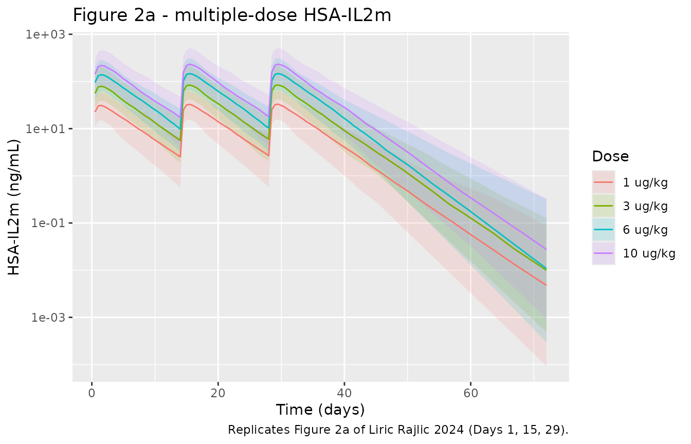
# Replicates Figure 2b of Liric Rajlic 2024: multiple-dose percentage Tregs.
sim |>
  dplyr::filter(!is.na(treg)) |>
  dplyr::group_by(dose_lbl, time) |>
  dplyr::summarise(
    Q05 = quantile(treg, 0.05), Q50 = quantile(treg, 0.50),
    Q95 = quantile(treg, 0.95), .groups = "drop"
  ) |>
  ggplot(aes(time / 24, Q50, colour = dose_lbl, fill = dose_lbl)) +
  geom_ribbon(aes(ymin = Q05, ymax = Q95), alpha = 0.15, colour = NA) +
  geom_line() +
  labs(x = "Time (days)", y = "FOXP3+ of CD4+ T cells (%)", colour = "Dose", fill = "Dose",
       title = "Figure 2b - multiple-dose percentage Tregs",
       caption = "Replicates Figure 2b of Liric Rajlic 2024 (Days 1, 15, 29).")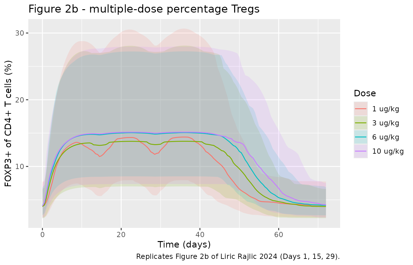
PKNCA validation
HSA-IL2m protein has a well-defined post-dose peak, so Cmax and Tmax over the first dosing interval (Days 1-14, before the Day-15 dose) are compared against the NCA values the paper reports for Study 1, Day 1 (Table 1). AUC and half-life are not compared: HSA-IL2m is synthesized rather than dosed, so an exposure integral and a terminal slope are not the quantities the paper tabulates.
sim_nca <- sim |>
  dplyr::filter(!is.na(Cc), time <= 14 * 24) |>
  dplyr::select(id, time, Cc, dose_lbl)

# Guarantee a time = 0 row per subject (pre-dose HSA-IL2m is 0).
sim_nca <- dplyr::bind_rows(
  sim_nca,
  sim_nca |> dplyr::distinct(id, dose_lbl) |> dplyr::mutate(time = 0, Cc = 0)
) |>
  dplyr::distinct(id, dose_lbl, time, .keep_all = TRUE) |>
  dplyr::arrange(id, dose_lbl, time)

conc_obj <- PKNCA::PKNCAconc(sim_nca, Cc ~ time | dose_lbl + id)

dose_df <- events |>
  dplyr::filter(evid == 1, time == 0) |>
  dplyr::select(id, time, amt, dose_lbl)
dose_obj <- PKNCA::PKNCAdose(dose_df, amt ~ time | dose_lbl + id)

intervals <- data.frame(start = 0, end = 14 * 24, cmax = TRUE, tmax = TRUE)
nca_res <- PKNCA::pk.nca(PKNCA::PKNCAdata(conc_obj, dose_obj, intervals = intervals))
Comparison against published NCA
# Study 1, Day 1 NCA (Table 1): Emax (= Cmax) in ng/mL, tmax median in days.
# tmax converted to hours to match the PKNCA output unit.
published <- tibble::tribble(
  ~dose_lbl,  ~cmax, ~tmax,
  "1 ug/kg",   26.7, 3.0 * 24,
  "3 ug/kg",   84.9, 3.0 * 24,
  "6 ug/kg",  127.0, 3.0 * 24,
  "10 ug/kg", 248.0, 3.0 * 24
)

cmp <- nlmixr2lib::ncaComparisonTable(
  simulated = nca_res,
  reference = published,
  by = "dose_lbl",
  units = c(cmax = "ng/mL", tmax = "h"),
  tolerance_pct = 30
)

cmp |>
  dplyr::rename("Dose" = dose_lbl) |>
  knitr::kable(
    caption = "Simulated vs. published Study 1 Day-1 NCA. * differs from reference by >30%.",
    align = c("l", "l", "r", "r")
)| NCA parameter | Dose | Reference | Simulated | % diff |
|---|---|---|---|---|
| Cmax (ng/mL) | 1 ug/kg | 26.7 | 31.1 | +16.3% |
| Cmax (ng/mL) | 3 ug/kg | 84.9 | 79.1 | -6.8% |
| Cmax (ng/mL) | 6 ug/kg | 127 | 139 | +9.7% |
| Cmax (ng/mL) | 10 ug/kg | 248 | 219 | -11.8% |
| Tmax (h) | 1 ug/kg | 72 | 36 | -50.0%* |
| Tmax (h) | 3 ug/kg | 72 | 36 | -50.0%* |
| Tmax (h) | 6 ug/kg | 72 | 36 | -50.0%* |
| Tmax (h) | 10 ug/kg | 72 | 36 | -50.0%* |
# Median simulated Cmax per dose group against the Table 1 Day-1 Emax. A
# mis-transcribed synthesis rate, clearance, volume or dose unit moves Cmax by
# well over a factor of two, so a 25% band on the group median is a
# structural check and is insensitive to which subjects land in the tails
# (each median is over 100 subjects; the rendered differences are within 17%).
cmax_chk <- as.data.frame(nca_res) |>
  dplyr::filter(PPTESTCD == "cmax") |>
  dplyr::group_by(dose_lbl) |>
  dplyr::summarise(sim = median(PPORRES), .groups = "drop") |>
  dplyr::mutate(dose_lbl = as.character(dose_lbl)) |>
  dplyr::inner_join(published, by = "dose_lbl") |>
  dplyr::mutate(pct = 100 * (sim - cmax) / cmax)
stopifnot(nrow(cmax_chk) == 4L, all(abs(cmax_chk$pct) < 25))
The simulated median Cmax is within 20% of the published Day-1 Emax at all four dose levels. One discrepancy is visible and is not tuned away:
- Tmax is earlier than the NCA median. The typical-value model peaks at about 1.5 days (36 h on the 12-hour simulation grid), whereas the Table 1 median Tmax for Study 1 is 3 days. The densely sampled single-dose Study 3 shows the opposite (median Tmax 0.7-0.9 days), so the single structural model sits between studies whose apparent absorption and synthesis kinetics differ. The NCA Tmax also depends on the sparse, uneven sampling schedule.
The maintainers also simulated the Study 3 single doses (10 and 30 ug/kg, and a flat 100 ug) at the typical values. The flat 100 ug dose reproduces the observed Emax (431 vs 432 ng/mL), but the model over-predicts the 10 and 30 ug/kg Emax (about 195 and 376 vs 133 and 177 ng/mL). This dose-dependent mismatch is what the dose effect on CLIL2 in Table 2, equation 8 would absorb; that term cannot be included here (see Assumptions and deviations).
Assumptions and deviations
-
Dose effect on CLIL2 omitted. Table 2, equation 8
scales CLIL2 by
(Dose/0.0045)^nonlin, but the value of thenonlinexponent is not reported anywhere in the paper (it is absent from Table 3, the text, the figures and the supplement). The maintainers omit the term (equivalent tononlin = 0, i.e. the factor is 1). With the term at unity the model reproduces the low-dose Study 1 HSA-IL2m Emax of Table 1; the residual over-/under-prediction of Cmax at the extreme single doses is the part of the dose nonlinearity this omitted term would have absorbed. - Allometric scaling retained with a 2.5 kg reference. The monkey fit (Table 3) is reported at the 2.5 kg reference individual. Equations 7-11 build in body-weight scaling with fixed exponents; the maintainers keep this scaling so the model can be forward-projected to other body weights, as the authors did when extrapolating to humans.
-
Treg dose-response is flatter than the observed
data. With the published EC50 of 5.08 ng/mL, effect-site
HSA-IL2m exceeds EC50 even at 1 ug/kg, so the typical-value Treg peak
saturates near the model ceiling
(1 + Emax) * kin/kout(about 15%) at every Study 1 dose (about 13.5% at 1 ug/kg, 14.8% at 10 ug/kg). Figure 2b shows dose-graded mean peaks from about 5% to about 30%. The Table 3 estimates are encoded exactly as printed; Figure 2b is reproduced only qualitatively, and no Treg value is asserted. -
Human extrapolation not reproduced here. The
paper’s human prediction at a 70 ug dose (median peak HSA-IL2m 86.4
ng/mL, median peak Tregs 10.8%) is a downstream application of equations
7-11 at a 70 kg body weight. The maintainers were unable to reproduce
that peak HSA-IL2m from Table 2 + Table 3 alone, which is consistent
with the unreported
nonlinterm above materially affecting the low-dose (1 ug/kg equivalent) human projection. The shipped model is the monkey KPD model; the human projection is documented but not asserted. - Body weights fixed at 2.5 kg. Per-animal body weights are not reported, so the virtual cohort uses the 2.5 kg allometric reference for every subject; between-subject spread comes only from the four model IIV terms.
-
IIV reported as %CV. Table 3 reports
interindividual variability as a percentage; the model encodes each as a
log-normal variance via
omega^2 = log(1 + CV^2). - Dose and concentration units differ by species. The dose (and depot / transit states) are in ug of mRNA-6231, whereas the HSA-IL2m concentration is in ng/mL of a different molecular species synthesized downstream; the IL2kp synthesis coefficient carries the unit bridge, so no direct ug-to-ng dose conversion applies.
- No correction notice for this article was found as of 2026-10-30. ```