Hydroxychloroquine in cynomolgus macaques (Liu 2020)
Source:vignettes/articles/Liu_2020_hydroxychloroquine_monkey.Rmd
Liu_2020_hydroxychloroquine_monkey.RmdModel and source
- Citation: Liu Q, Bi G, Chen G, Guo X, Tu S, Tong X, Xu M, Liu M, Wang B, Jiang H, Wang J, Li H, Wang K, Liu D, Song C. Time-Dependent Distribution of Hydroxychloroquine in Cynomolgus Macaques Using Population Pharmacokinetic Modeling Method. Front Pharmacol. 2021;11:602880. doi:10.3389/fphar.2020.602880. PMCID: PMC7841297. Structural model: Equations 1-8 and Figure 2 (Methods, ‘Structural PK Model’). Parameter estimates and between-animal variability: Table 4. Error model and estimation method: Methods, ‘Structural PK Model’ and ‘Software and Platform Used’.
- Description: Preclinical (cynomolgus macaque). Five-compartment population PK model of oral (intragastric) hydroxychloroquine fitted jointly to plasma, whole-blood and lung-tissue concentrations in 17 male cynomolgus macaques. First-order absorption from a depot into a central (plasma) compartment with first-order elimination (Ke) and a linear exchange with an unobserved peripheral compartment (Kcp / Kpc). Transfer from the central compartment into a red-blood-cell compartment and into a lung-tissue compartment is saturable in the central AMOUNT (Kmax * A1 / (A50 + A1), Acb50 = 7.05 mg and Acl50 = 0.498 mg), with first-order return to the central compartment (Kbc, Klc). The whole-blood concentration is the sum of the red-cell and plasma concentrations (A3 / Vb + A1 / Vc). Fitted by the MLEM algorithm in ADAPT 5 with log-normal between-animal variability on all 13 structural parameters and a proportional-plus-additive residual error per matrix. The printed parameters reproduce the observed single-dose (3 mg/kg) whole-blood and plasma NCA and the paper’s own population predictions for lung (Figure 5B), but not its simulated Figure 9 / Table 5 profiles, whose regimen is unstated (see the vignette).
- Article: https://doi.org/10.3389/fphar.2020.602880 (open access; PMC7841297)
Read this first: two of the paper’s printed artefacts do not match the model’s own predictions. Table 4 and Equations 1-8 are encoded exactly as printed. With them the model reproduces the observed single-dose (3 mg/kg) whole-blood and plasma NCA reported in the Results. It also reproduces, to within 3%, the paper’s own population predictions for the lung samples of groups E and F (Figure 5B). It does not reproduce the simulated Figure 9 and Table 5. There the simulated lung concentrations sit a uniform ~2-fold above Table 5, although their terminal decline matches. The Figure 9 regimen is not stated, but the lung plateau is saturable and almost independent of dose, so no choice of regimen closes the gap. Separately, the lung concentrations the model was fitted to (Figure 5) are 8- to 11-fold higher than the lung means printed in Table 1. The paper’s own tissue-to-blood and tissue-to-plasma ratios agree with the Figure 5 scale, not with Table 1. Details are in the sections below, and the gates hold these findings so that a later change to the model shows up.
Population
Seventeen male cynomolgus macaques (4.13 +/- 0.43 kg) received hydroxychloroquine intragastrically in six regimens between 1 and 21 mg/kg, over 1 to 5 days (Methods, “Pharmacokinetics Analysis” and “Subjects and Study Design”). Doses given on the same day were 4 h apart. The model was fitted jointly to 141 plasma samples, 149 whole-blood samples and one terminal lung sample in 14 of the 17 animals, taken at necropsy between 120 and 504 h after the first dose. The same information is available programmatically:
str(readModelDb("Liu_2020_hydroxychloroquine_monkey")()$population)
#> List of 9
#>  $ species       : chr "cynomolgus macaque (Macaca fascicularis)"
#>  $ n_subjects    : int 17
#>  $ n_studies     : int 1
#>  $ sex_female_pct: num 0
#>  $ weight_range  : chr "4.13 +/- 0.43 kg (mean +/- SD; Methods, 'Experimental Animals')"
#>  $ disease_state : chr "Healthy animals (biodistribution study motivated by COVID-19 repurposing of hydroxychloroquine)"
#>  $ dose_range    : chr "Hydroxychloroquine 1-21 mg/kg intragastrically, in six regimens: single 3 mg/kg; 3 mg/kg twice 4 h apart on day"| __truncated__
#>  $ regions       : chr "China (Pharmaron Beijing Co., Ltd.; Peking University Third Hospital)"
#>  $ notes         : chr "Six groups (n = 3 each, except group F n = 2), all male. 141 plasma and 149 whole-blood samples (intensive samp"| __truncated__
Source trace
Every ini() value carries an in-file comment pointing to
its source. The table below collects them.
| Equation / parameter | Value | Source location |
|---|---|---|
| Central (plasma) amount, Equation 1 | d/dt(central) |
Equation 1; Figure 2 |
| Depot, Equation 2 | d/dt(depot) = -ka * depot |
Equation 2 |
| Red-cell compartment, Equation 3 | d/dt(rbc_hcq) |
Equation 3; Figure 2 |
| Lung compartment, Equation 4 | d/dt(lung) |
Equation 4; Figure 2 |
| Peripheral compartment, Equation 5 | d/dt(peripheral1) |
Equation 5 |
| Plasma / whole-blood / lung concentration |
Cc, Cblood, Clung
|
Equations 6-8 |
lka (Ka) |
log(0.592 1/h) | Table 4 |
lkel (Ke) |
log(0.236 1/h) | Table 4 |
lvc (Vc/F) |
log(114 L) | Table 4 |
lk12 (Kcp) |
log(0.600 1/h) | Table 4 |
lk21 (Kpc) |
log(0.514 1/h) | Table 4 |
lvmax_rbc (Kcbmax) |
log(2.48 mg/h) | Table 4 (unit: see Assumptions) |
lkm_rbc (Acb50) |
log(7.05 mg) | Table 4 |
lkeff_rbc (Kbc) |
log(0.718 1/h) | Table 4 |
lv_rbc (Vb/F) |
log(2.68 L) | Table 4 |
lvmax_lung (Kclmax) |
log(1.92 mg/h) | Table 4 (unit: see Assumptions) |
lkm_lung (Acl50) |
log(0.498 mg) | Table 4 |
lk_lung_central (Klc) |
log(0.159 1/h) | Table 4 |
lv_lung (VL/F) |
log(5.55 L) | Table 4 |
13 eta variances |
log(1 + CV^2) from the IIV CV% column | Table 4 |
propSd, propSd_Cblood,
propSd_Clung
|
0.286, 0.118, 0.0514 | Table 4 (PD pl, PD bl, PD lu) |
addSd, addSd_Cblood,
addSd_Clung
|
1e-5, fixed | Table 4 (SD pl, SD bl, SD lu) |
| Residual form | proportional plus additive (combined1) |
Methods, “Structural PK Model” and “Software and Platform Used” |
Model setup
mod <- rxode2::rxode2(readModelDb("Liu_2020_hydroxychloroquine_monkey"))
#> ℹ parameter labels from comments will be replaced by 'label()'
mod_typ <- rxode2::zeroRe(mod)
# The explicit ODEs must be solved as written (no linear-compartment
# auto-solve replacing them).
stopifnot(is.null(mod$linCmt))

wt <- 4.13 # kg, mean body weight (Methods)
Doses are given in mg as mg/kg multiplied by the 4.13 kg mean body
weight. All observation records sit on the central state
with dvid = 1. The model declares three error endpoints, so
every observation row has to name one, and Cc,
Cblood and Clung are all returned as columns
at each of those records.
# One event table per regimen. `doses` is a data frame of time (h) and
# dose (mg/kg); observations are on the central state.
make_events <- function(doses, obs_times, id = 1L, regimen = "") {
  dose_rows <- data.frame(
    id = id, time = doses$time, amt = doses$mgkg * wt,
    evid = 1L, cmt = "depot", dvid = NA_integer_
  )
  obs_rows <- data.frame(
    id = id, time = obs_times, amt = 0, evid = 0L, cmt = "central", dvid = 1L
  )
  out <- dplyr::bind_rows(dose_rows, obs_rows) |>
    dplyr::arrange(id, time, dplyr::desc(evid))
  out$regimen <- regimen
  out
}

# rxSolve() omits the `id` column when only one subject is solved; restore it.
solve_df <- function(model, events) {
  out <- as.data.frame(rxode2::rxSolve(model, events, keep = "regimen"))
  if (!"id" %in% names(out)) out$id <- 1L
  out
}

regimens <- list(
  "3 mg/kg single" = data.frame(time = 0, mgkg = 3),
  "3 mg/kg x2 on days 1-2" = data.frame(time = c(0, 4, 24, 28), mgkg = 3),
  "2 mg/kg x2 then 1 mg/kg x2 daily" = data.frame(
    time = c(0, 4, 24, 28, 48, 52), mgkg = c(2, 2, 1, 1, 1, 1)
  ),
  "6 mg/kg x2 then 2 mg/kg x2 daily" = data.frame(
    time = c(0, 4, 24, 28, 48, 52), mgkg = c(6, 6, 2, 2, 2, 2)
  ),
  "21 mg/kg x2 (group E)" = data.frame(time = c(0, 4), mgkg = 21),
  "21 mg/kg x2 then 7 mg/kg x2 daily (group F)" = data.frame(
    time = c(0, 4, 24, 28, 48, 52, 72, 76, 96, 100),
    mgkg = c(21, 21, rep(7, 8))
  )
)
Replicate Figure 1: observed-design regimens
Figure 1 of the paper shows the observed whole-blood and plasma concentrations for the six regimens. The typical-value predictions for the same designs are below. The sampling windows are 72 h for the four low-dose groups, 264 h for group E and 120 h for group F.
end_time <- c(72, 72, 72, 72, 264, 120)
ev_fig1 <- dplyr::bind_rows(lapply(seq_along(regimens), function(i) {
  make_events(
    regimens[[i]], seq(0, end_time[i], by = 0.5),
    id = i, regimen = names(regimens)[i]
  )
}))
sim_fig1 <- solve_df(mod_typ, ev_fig1)
#> ℹ omega/sigma items treated as zero: 'etalka', 'etalkel', 'etalvc', 'etalk12', 'etalk21', 'etalvmax_rbc', 'etalkm_rbc', 'etalkeff_rbc', 'etalv_rbc', 'etalvmax_lung', 'etalkm_lung', 'etalk_lung_central', 'etalv_lung'
#> Warning: multi-subject simulation without without 'omega'

# Drop the pre-dose zero so it does not break the log axis.
sim_fig1[sim_fig1$time != 0, ] |>
  tidyr::pivot_longer(c(Cc, Cblood), names_to = "matrix", values_to = "conc") |>
  dplyr::mutate(matrix = dplyr::recode(matrix, Cc = "Plasma", Cblood = "Whole blood")) |>
  ggplot(aes(time, conc, colour = regimen)) +
  geom_line() +
  facet_wrap(~matrix) +
  scale_y_log10() +
  labs(
    x = "Time after first dose (h)", y = "HCQ concentration (ng/mL)",
    colour = NULL,
    caption = "Typical-value predictions for the regimens of Figure 1 of Liu 2020."
  ) +
  theme(legend.position = "bottom") +
  guides(colour = guide_legend(ncol = 2))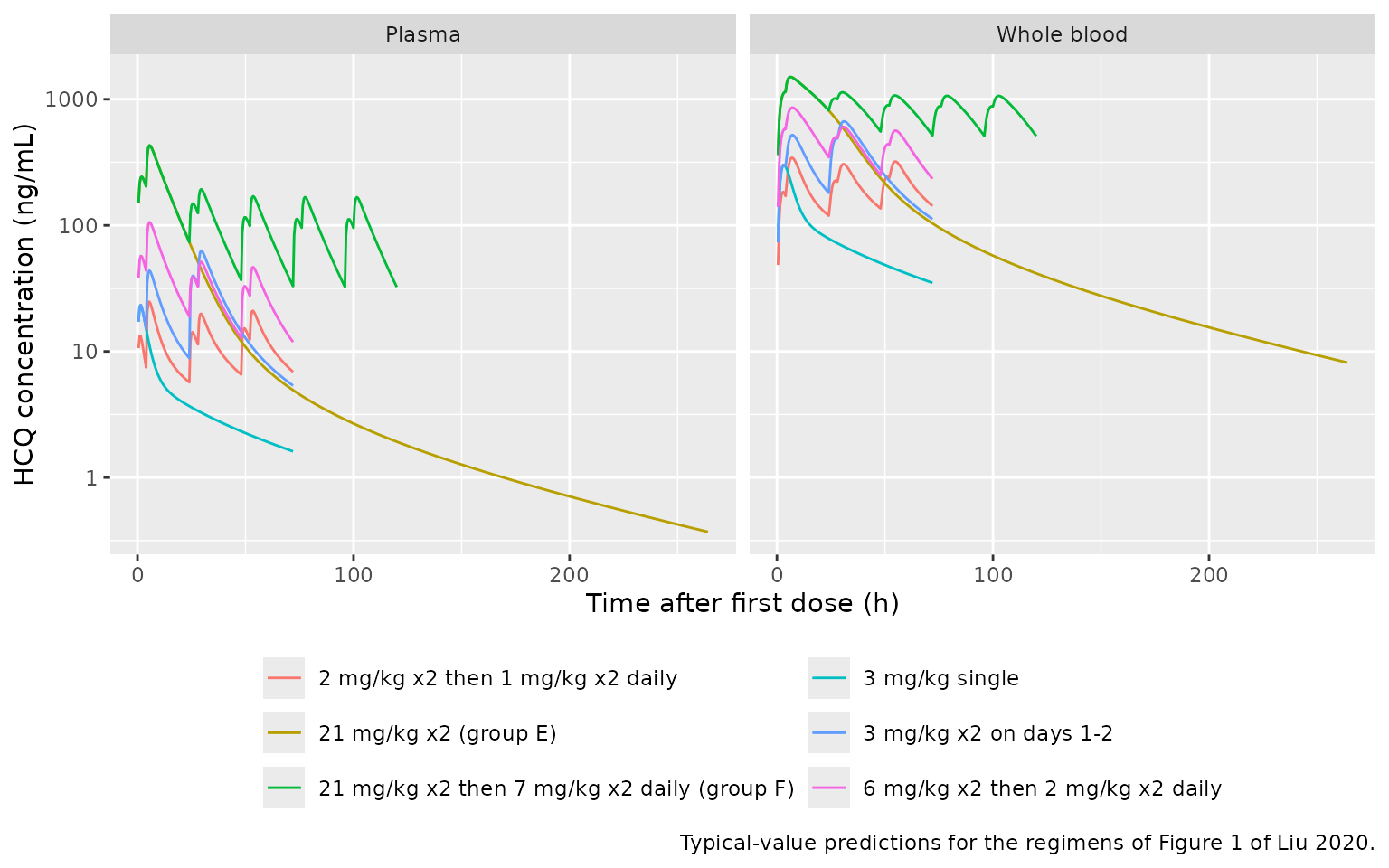
Single-dose NCA against the observed data
The Results report the NCA from WinNonlin after a single 3 mg/kg dose, with blood and plasma sampled at 0, 1, 2, 4, 8, 24, 48 and 72 h. Cmax was 292.33 +/- 114.66 ng/mL in blood and 36.90 +/- 22.52 ng/mL in plasma. AUC0-inf was 5,978.94 +/- 1,981.30 h*ng/mL in blood and 363.31 +/- 195.38 h*ng/mL in plasma. The simulated profiles are put through PKNCA on the same sampling times, so AUC0-inf is extrapolated from a 72 h profile in the same way as the observed value.
nca_times <- c(0, 1, 2, 4, 8, 24, 48, 72)
sd_dose <- regimens[["3 mg/kg single"]]

# Typical-value animal (deterministic).
ev_typ <- make_events(sd_dose, nca_times, id = 1L, regimen = "3 mg/kg single")
sim_typ <- solve_df(mod_typ, ev_typ)
#> ℹ omega/sigma items treated as zero: 'etalka', 'etalkel', 'etalvc', 'etalk12', 'etalk21', 'etalvmax_rbc', 'etalkm_rbc', 'etalkeff_rbc', 'etalv_rbc', 'etalvmax_lung', 'etalkm_lung', 'etalk_lung_central', 'etalv_lung'

# Stochastic cohort for the between-animal spread (100 animals).
rxode2::rxSetSeed(20201116)
n_anim <- 100L
ev_coh <- dplyr::bind_rows(lapply(seq_len(n_anim), function(i) {
  make_events(sd_dose, nca_times, id = i, regimen = "3 mg/kg single")
}))
sim_coh <- solve_df(mod, ev_coh)
run_nca <- function(sim, conc_col) {
  conc_df <- sim |>
    dplyr::transmute(id, time, treatment = regimen, conc = .data[[conc_col]]) |>
    dplyr::filter(!is.na(conc))
  dose_df <- data.frame(
    id = unique(conc_df$id), time = 0, treatment = "3 mg/kg single",
    amt = 3 * wt
  )
  conc_obj <- PKNCA::PKNCAconc(conc_df, conc ~ time | treatment + id)
  dose_obj <- PKNCA::PKNCAdose(dose_df, amt ~ time | treatment + id)
  intervals <- data.frame(
    start = 0, end = Inf, cmax = TRUE, tmax = TRUE,
    auclast = TRUE, aucinf.obs = TRUE, half.life = TRUE
  )
  res <- PKNCA::pk.nca(PKNCA::PKNCAdata(conc_obj, dose_obj, intervals = intervals))
  as.data.frame(res$result)
}

nca_typ <- dplyr::bind_rows(
  run_nca(sim_typ, "Cc") |> dplyr::mutate(matrix = "Plasma"),
  run_nca(sim_typ, "Cblood") |> dplyr::mutate(matrix = "Whole blood")
)
nca_coh <- dplyr::bind_rows(
  run_nca(sim_coh, "Cc") |> dplyr::mutate(matrix = "Plasma"),
  run_nca(sim_coh, "Cblood") |> dplyr::mutate(matrix = "Whole blood")
)
observed <- data.frame(
  matrix = c("Plasma", "Whole blood"),
  cmax = c(36.90, 292.33),
  aucinf.obs = c(363.31, 5978.94)
)

cmp_typ <- nlmixr2lib::ncaComparisonTable(
  simulated = nca_typ, reference = observed, by = "matrix",
  params = c("cmax", "aucinf.obs"),
  units = c(cmax = "ng/mL", aucinf.obs = "h*ng/mL")
)
cmp_coh <- nlmixr2lib::ncaComparisonTable(
  simulated = nca_coh, reference = observed, by = "matrix",
  params = c("cmax", "aucinf.obs"),
  units = c(cmax = "ng/mL", aucinf.obs = "h*ng/mL")
)

knitr::kable(
  cmp_typ,
  caption = "Typical-value animal vs. observed mean (n = 3), 3 mg/kg single dose."
)| NCA parameter | matrix | Reference | Simulated | % diff |
|---|---|---|---|---|
| Cmax (ng/mL) | Plasma | 36.9 | 22.6 | -38.8%* |
| Cmax (ng/mL) | Whole blood | 292 | 293 | +0.1% |
| AUC0-∞ (obs) (h*ng/mL) | Plasma | 363 | 413 | +13.6% |
| AUC0-∞ (obs) (h*ng/mL) | Whole blood | 5980 | 8350 | +39.7%* |
knitr::kable(
  cmp_coh,
  caption = "Median of 100 simulated animals vs. observed mean (n = 3), 3 mg/kg single dose."
)| NCA parameter | matrix | Reference | Simulated | % diff |
|---|---|---|---|---|
| Cmax (ng/mL) | Plasma | 36.9 | 19.4 | -47.3%* |
| Cmax (ng/mL) | Whole blood | 292 | 245 | -16.3% |
| AUC0-∞ (obs) (h*ng/mL) | Plasma | 363 | 375 | +3.1% |
| AUC0-∞ (obs) (h*ng/mL) | Whole blood | 5980 | 5840 | -2.4% |
- differs from reference by more than ±20%.
The median of the simulated cohort reproduces both observed AUC0-inf values and the whole-blood Cmax. Its plasma Cmax sits below the observed mean, but well inside the observed +/- 1 SD range (14.4 to 59.4 ng/mL). An observed mean of three animals, with a 61% CV on Cmax, is a weak reference for any single number.
The typical-value animal is not the cohort median here. The red-cell and lung transfers saturate, and their parameters carry CVs above 100%, so the median of the simulated profiles sits away from the profile of the median animal. The typical animal’s terminal phase is also slower than the observed one: extrapolation beyond 72 h makes up about a quarter of its whole-blood AUC0-inf, where the paper reports under 10% for blood and under 20% for plasma. Its AUC0-inf therefore overshoots. Its AUC0-72 needs no extrapolation. For plasma it lies inside the range implied by the reported AUC0-inf and extrapolated share, and for whole blood it lies about 5% above that range.
typ_val <- function(mat, code) {
  v <- nca_typ$PPORRES[nca_typ$matrix == mat & nca_typ$PPTESTCD == code]
  if (length(v) != 1L) stop("no unique NCA value for ", mat, " ", code)
  v
}
coh_med <- function(mat, code) {
  v <- nca_coh$PPORRES[nca_coh$matrix == mat & nca_coh$PPTESTCD == code]
  if (length(v) != n_anim) stop("expected one value per animal for ", mat, " ", code)
  median(v, na.rm = TRUE)
}
# Observed AUC0-72 implied by the reported AUC0-inf and the reported
# extrapolated share (< 20% plasma, < 10% blood; Results).
auc72_range <- rbind(
  Plasma = c(0.80, 1.00) * 363.31,
  `Whole blood` = c(0.90, 1.00) * 5978.94
)
gate_tab <- data.frame(
  Quantity = c(
    "Typical: plasma Cmax (ng/mL)", "Typical: whole-blood Cmax (ng/mL)",
    "Typical: plasma AUC0-72 (h*ng/mL)", "Typical: whole-blood AUC0-72 (h*ng/mL)",
    "Typical: whole-blood extrapolated share of AUC0-inf (%)",
    "Cohort median: plasma AUC0-inf (h*ng/mL)", "Cohort median: whole-blood AUC0-inf (h*ng/mL)"
  ),
  Simulated = c(
    typ_val("Plasma", "cmax"), typ_val("Whole blood", "cmax"),
    typ_val("Plasma", "auclast"), typ_val("Whole blood", "auclast"),
    100 * (1 - typ_val("Whole blood", "auclast") / typ_val("Whole blood", "aucinf.obs")),
    coh_med("Plasma", "aucinf.obs"), coh_med("Whole blood", "aucinf.obs")
  ),
  Observed = c(
    "36.90 +/- 22.52", "292.33 +/- 114.66",
    "290.6 to 363.3 (implied)", "5381 to 5979 (implied)", "< 10",
    "363.31 +/- 195.38", "5978.94 +/- 1981.30"
  )
)
knitr::kable(gate_tab, digits = 1, caption = "Gated quantities, 3 mg/kg single dose.")| Quantity | Simulated | Observed |
|---|---|---|
| Typical: plasma Cmax (ng/mL) | 22.6 | 36.90 +/- 22.52 |
| Typical: whole-blood Cmax (ng/mL) | 292.6 | 292.33 +/- 114.66 |
| Typical: plasma AUC0-72 (h*ng/mL) | 319.2 | 290.6 to 363.3 (implied) |
| Typical: whole-blood AUC0-72 (h*ng/mL) | 6269.0 | 5381 to 5979 (implied) |
| Typical: whole-blood extrapolated share of AUC0-inf (%) | 24.9 | < 10 |
| Cohort median: plasma AUC0-inf (h*ng/mL) | 374.8 | 363.31 +/- 195.38 |
| Cohort median: whole-blood AUC0-inf (h*ng/mL) | 5837.5 | 5978.94 +/- 1981.30 |
stopifnot(
  # Deterministic typical-value animal. A mis-transcribed volume, rate or
  # unit moves these by tens of percent.
  typ_val("Plasma", "cmax") > 36.90 - 22.52,
  typ_val("Plasma", "cmax") < 36.90 + 22.52,
  abs(typ_val("Whole blood", "cmax") / 292.33 - 1) < 0.15,
  typ_val("Plasma", "auclast") > 0.9 * auc72_range["Plasma", 1],
  typ_val("Plasma", "auclast") < 1.1 * auc72_range["Plasma", 2],
  typ_val("Whole blood", "auclast") > 0.9 * auc72_range["Whole blood", 1],
  typ_val("Whole blood", "auclast") < 1.1 * auc72_range["Whole blood", 2],
  # Cohort median (100 animals): the centre, with headroom for the draw.
  abs(coh_med("Plasma", "aucinf.obs") / 363.31 - 1) < 0.25,
  abs(coh_med("Whole blood", "aucinf.obs") / 5978.94 - 1) < 0.25
)
Lung: population predictions (Figure 5B) and Table 1
The lung data are single terminal samples from 14 animals. Figure 5B plots each observed lung concentration against the model’s population prediction (PRED). Groups E and F are the only groups necropsied at 264 h and 120 h, so their points can be identified unambiguously. The maintainers digitised the circle centres of Figure 5B from the published raster.
fig5b <- data.frame(
  group = c("F", "F", "E", "E", "E"),
  time = c(120, 120, 264, 264, 264),
  pred = c(1968.4, 2022.5, 167.3, 178.2, 181.5),
  obs = c(4875.4, 7731.1, 179.4, 348.7, 152.7)
)
lung_at <- function(reg, t_obs) {
  s <- sim_fig1[sim_fig1$regimen == reg & sim_fig1$time == t_obs, ]
  if (nrow(s) != 1L) stop("no unique row for ", reg, " at ", t_obs, " h")
  s
}
sF <- lung_at("21 mg/kg x2 then 7 mg/kg x2 daily (group F)", 120)
sE <- lung_at("21 mg/kg x2 (group E)", 264)

lung_tab <- fig5b |>
  dplyr::group_by(group, time) |>
  dplyr::summarise(
    fig5b_pred = mean(pred), fig5b_obs = mean(obs), .groups = "drop"
  ) |>
  dplyr::mutate(
    sim_typical = c(E = sE$Clung, F = sF$Clung)[group],
    table1_mean = c(E = 20.77, F = 738.50)[group],
    sim_over_pred = sim_typical / fig5b_pred,
    fig5b_obs_over_table1 = fig5b_obs / table1_mean
  )
lung_tab |>
  dplyr::rename(
    Group = group, `Time (h)` = time,
    `Figure 5B PRED (ng/g)` = fig5b_pred,
    `Figure 5B observed (ng/g)` = fig5b_obs,
    `Simulated typical (ng/g)` = sim_typical,
    `Table 1 mean (ng/g)` = table1_mean,
    `Simulated / PRED` = sim_over_pred,
    `Figure 5B observed / Table 1` = fig5b_obs_over_table1
  ) |>
knitr::kable(digits = 2, caption = "Lung: typical-value prediction vs. Figure 5B (digitised) and Table 1.")| Group | Time (h) | Figure 5B PRED (ng/g) | Figure 5B observed (ng/g) | Simulated typical (ng/g) | Table 1 mean (ng/g) | Simulated / PRED | Figure 5B observed / Table 1 |
|---|---|---|---|---|---|---|---|
| E | 264 | 175.67 | 226.93 | 180.29 | 20.77 | 1.03 | 10.93 |
| F | 120 | 1995.45 | 6303.25 | 1998.19 | 738.50 | 1.00 | 8.54 |
The typical-value animal reproduces the paper’s population predictions for both groups. That confirms the transcription of the lung parameters, the saturable-transfer form and the concentration scale. The paper’s PRED underpredicts the group F observations about 3-fold, and so does this model. That is a property of the published fit, not of this implementation.
The observed values in Figure 5 are 8- to 11-fold higher than the means in Table 1. The Methods homogenise each tissue with ten volumes of 50% methanol, and the Table 1 values look like homogenate concentrations that were not corrected for that dilution. Two things support this. The Kp ratios printed next to them in Tables 1 and 3 are consistent with the Figure 5 scale. And 10 x 738.50 ng/g divided by the ~27 ng/mL group F plasma level read from Figure 1C gives about 270, against the printed lung-to-plasma Kp of 267.38. This is an interpretation; the paper does not state it. The model is compared here with Figure 5, the data it was fitted to.
# Deterministic typical-value predictions against the digitised PRED.
# Realised: 1.00 (group F) and 1.03 (group E). Digitising error is about 2%.
stopifnot(
  nrow(lung_tab) == 2L,
  all(abs(lung_tab$sim_over_pred - 1) < 0.08),
  # The documented Table 1 scale gap.
  all(lung_tab$fig5b_obs_over_table1 > 7), all(lung_tab$fig5b_obs_over_table1 < 12)
)
Replicate Figure 9 and Table 5: simulated multiple-dose profile
The paper simulates “one dosing regimen” with the typical parameters, and Table 5 reports concentrations at 12 to 96 h after the last dose. The regimen is not stated. Figure 9 shows two 12-hourly loading doses and then eight 12-hourly maintenance doses (last dose at 108 h). The regimen below uses group F’s dose levels (21 mg/kg, then 7 mg/kg) on that 12-hourly schedule. This is an assumption for illustration only.
fig9_doses <- data.frame(time = seq(0, 108, by = 12), mgkg = c(21, 21, rep(7, 8)))
tab5 <- data.frame(
  tad = c(12, 24, 48, 72, 96),
  Cc = c(10.63, 4.26, 1.80, 1.10, 0.76),
  Cblood = c(187.29, 85.40, 37.68, 23.19, 16.11),
  Clung = c(1008.54, 865.68, 629.94, 482.23, 380.55)
)
ev9 <- make_events(
  fig9_doses, sort(unique(c(seq(0, 348, by = 0.5), 108 + tab5$tad))),
  regimen = "Figure 9 (assumed)"
)
sim9 <- solve_df(mod_typ, ev9)
#> ℹ omega/sigma items treated as zero: 'etalka', 'etalkel', 'etalvc', 'etalk12', 'etalk21', 'etalvmax_rbc', 'etalkm_rbc', 'etalkeff_rbc', 'etalv_rbc', 'etalvmax_lung', 'etalkm_lung', 'etalk_lung_central', 'etalv_lung'

sim9 |>
  tidyr::pivot_longer(c(Cc, Cblood, Clung), names_to = "matrix", values_to = "conc") |>
  dplyr::mutate(matrix = factor(
    matrix, c("Cc", "Cblood", "Clung"),
    c("Plasma (ng/mL)", "Whole blood (ng/mL)", "Lung (ng/g)")
  )) |>
  ggplot(aes(time, conc)) +
  geom_line() +
  geom_point(
    data = tab5 |>
      tidyr::pivot_longer(-tad, names_to = "matrix", values_to = "conc") |>
      dplyr::mutate(
        time = 108 + tad,
        matrix = factor(
          matrix, c("Cc", "Cblood", "Clung"),
          c("Plasma (ng/mL)", "Whole blood (ng/mL)", "Lung (ng/g)")
        )
      ),
    colour = "red"
  ) +
  facet_wrap(~matrix, scales = "free_y") +
  scale_y_log10() +
  labs(
    x = "Time (h)", y = "HCQ concentration",
    caption = "Line: typical-value simulation, assumed regimen. Red points: Table 5 of Liu 2020."
  )
#> Warning in scale_y_log10(): log-10 transformation introduced infinite values.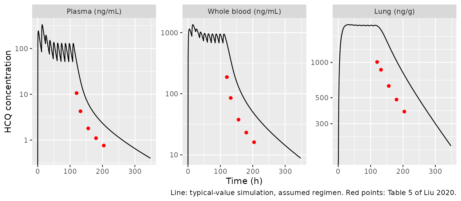
sim_tab5 <- sim9[match(108 + tab5$tad, sim9$time), c("Cc", "Cblood", "Clung")]
stopifnot(nrow(sim_tab5) == 5L, !anyNA(sim_tab5))
tab5_cmp <- data.frame(
  `TAD (h)` = tab5$tad,
  `Plasma, Table 5` = tab5$Cc, `Plasma, sim` = sim_tab5$Cc,
  `Blood, Table 5` = tab5$Cblood, `Blood, sim` = sim_tab5$Cblood,
  `Lung, Table 5` = tab5$Clung, `Lung, sim` = sim_tab5$Clung,
  `Lung/plasma, Table 5` = tab5$Clung / tab5$Cc,
  `Lung/plasma, sim` = sim_tab5$Clung / sim_tab5$Cc,
  check.names = FALSE
)
knitr::kable(tab5_cmp, digits = 2, caption = "Table 5 of Liu 2020 vs. the typical-value simulation (assumed regimen).")| TAD (h) | Plasma, Table 5 | Plasma, sim | Blood, Table 5 | Blood, sim | Lung, Table 5 | Lung, sim | Lung/plasma, Table 5 | Lung/plasma, sim |
|---|---|---|---|---|---|---|---|---|
| 12 | 10.63 | 51.57 | 187.29 | 677.77 | 1008.54 | 2051.95 | 94.88 | 39.79 |
| 24 | 4.26 | 19.77 | 85.40 | 356.98 | 865.68 | 1895.71 | 203.21 | 95.90 |
| 48 | 1.80 | 6.26 | 37.68 | 130.00 | 629.94 | 1400.74 | 349.97 | 223.65 |
| 72 | 1.10 | 3.39 | 23.19 | 72.33 | 482.23 | 1029.43 | 438.39 | 303.55 |
| 96 | 0.76 | 2.19 | 16.11 | 47.19 | 380.55 | 780.01 | 500.72 | 356.76 |
The lung level sits about 2-fold above Table 5 at every time. The
lung decline over the same window matches: from 12 to 96 h after the
last dose, the simulated lung concentration falls by the same factor as
in Table 5. The saturable lung uptake makes the lung plateau
Kclmax / (Klc * VL), which is 2,176 ng/g with the printed
values, and the simulation approaches it during maintenance dosing.
Figure 9 shows a plateau of about 1,050 ng/g. The plasma and whole-blood
values depend on the unstated regimen and are not compared further.
lung_ratio <- sim_tab5$Clung / tab5$Clung
decline_sim <- sim_tab5$Clung[1] / sim_tab5$Clung[5]
decline_tab <- tab5$Clung[1] / tab5$Clung[5]
c(lung_ratio = round(lung_ratio, 3), decline_ratio = round(decline_sim / decline_tab, 3))
#>   lung_ratio1   lung_ratio2   lung_ratio3   lung_ratio4   lung_ratio5
#>         2.035         2.190         2.224         2.135         2.050
#> decline_ratio
#>         0.993
stopifnot(
  # Terminal lung decline: shape reproduced within 5%.
  abs(decline_sim / decline_tab - 1) < 0.05,
  # Lung level: the documented ~2-fold offset from Table 5.
  all(lung_ratio > 1.9), all(lung_ratio < 2.4),
  # Saturable lung plateau Kclmax / (Klc * VL), in ng/g.
  abs(1000 * 1.92 / (0.159 * 5.55) - 2175.8) < 1
)
Assumptions and deviations
-
Unit of Kcbmax and Kclmax. Table 4 prints no unit
for these two parameters, and the Results text gives them as h^-1.
Equation 1 and the Figure 2 arrows (
Kcbmax/(Acb50 + A1)multiplying A1) make the transfer fluxKmax * A1 / (A50 + A1)with A1 in mg, which needs Kmax in mg/h. The equation is followed. The only reading consistent with an h^-1 unit isKmax * A50 * A1 / (A50 + A1). For the lung term, that reading halves the flux, since Acl50 = 0.498 mg, and moves the lung plateau close to Figure 9. For the blood term it predicts a single-dose whole-blood Cmax about 5-fold above the observed value. It was therefore rejected. Nothing in the paper supports reading the two terms differently. - Typical values. The Table 4 “Mean” column is encoded as the typical (median) value. The paper refers to these estimates as the typical-monkey values (abstract) and uses the “typical parameters” for its simulations (Methods).
-
Between-animal variability. The IIV CV% is
converted to a log-normal variance as
omega^2 = log(1 + CV^2). ADAPT’s MLEM fits a multivariate log-normal distribution, but only the CVs are printed, so the covariance matrix is diagonal. The Results text says the CVs range “from 29 to 88.7%, except for IIV of Kcl (160%)”. Table 4 lists five CVs above 100% (Acb50, Vb/F, Acl50, Kcbmax, Kcp) and no parameter at 160%. Table 4 is used. -
Residual error. ADAPT’s proportional-plus-additive
model is
SD = SDinter + SDslope * Y, encoded ascombined1. The additive SDs are fixed at 1e-5, as printed, so the error is proportional in practice. - Lung concentration units. The lung amount in mg divided by VL in L gives mg/L, which is reported as ng/g assuming a tissue density of 1 g/mL.
- Dose units. Doses are in mg as reported. The paper does not say whether they are expressed as hydroxychloroquine sulfate (the administered material) or as base. Simulations use mg/kg x 4.13 kg, the mean body weight. The model has no body-size covariate.
- Group labels. The Figure 1 caption and the Methods text label the six groups differently. The dose levels and regimen shapes agree, and this vignette identifies regimens by dose, not by letter. The Tissue Distribution section’s group E and F labels are used for the lung data.
- Figure 9 / Table 5 regimen. Not stated in the paper. The regimen used here is an assumption, and the comparison with Table 5 is limited to the lung, whose plateau is set by the saturable uptake and not by the dose.
- Table 1 lung scale. The Table 1 tissue concentrations are compared only as a documented scale gap. The model is validated against the Figure 5B population predictions, which it reproduces.
- Known deviations. The printed parameters put the lung concentrations about 2-fold above the simulated Table 5 and Figure 9 values. The regimen behind those two artefacts is unknown. The paper’s own population prediction also underpredicts the group F lung observations about 3-fold. These deviations are recorded, not tuned away, and are held by the gates above.